simulationCases/coalescenceBubble.c
Coalescence of Bubbles
Axisymmetric simulation of two-bubble coalescence with size asymmetry using the Volume-of-Fluid (VOF) method. The simulation tracks the interface between gas (inside bubble, \(f=1\)) and liquid (outside, \(f=0\)) phases.
Scientific Context
This model isolates the hydrodynamic event responsible for electrolyte entrainment in gas-evolving electrochemical systems: coalescence between a large “parent” bubble and a smaller bubble. The key physical pathway is capillary-wave focusing on the smaller bubble that generates a Worthington jet and droplet pinch-off into the parent bubble.
Hydrodynamic Pathway (Captured Here)
- First contact creates a neck that expands rapidly.
- The neck launches capillary waves over the small bubble.
- Waves focus at the small bubble’s south pole.
- A Worthington jet forms and breaks up, injecting droplets into the gas.
Physical Setup
Two initially spherical bubbles of different sizes
are placed along the axis of symmetry. The smaller
bubble has radius 1 (reference scale), while the larger
bubble has radius Rr (the radius ratio
parameter). Surface tension drives the coalescence
dynamics.
Governing Equations
The incompressible Navier-Stokes equations with surface tension:
\[\nabla \cdot \mathbf{u} = 0\]
\[\rho\left(\frac{\partial \mathbf{u}}{\partial t} + \mathbf{u} \cdot \nabla \mathbf{u}\right) = -\nabla p + \nabla \cdot (2\mu \mathbf{D}) + \sigma \kappa \delta_s \mathbf{n}\]
where \(\mathbf{D}\) is the strain-rate tensor, \(\sigma\) is surface tension, \(\kappa\) is interface curvature, and \(\delta_s\) is the interface delta function.
Usage
./coalescenceBubble <OhOut> <RhoIn> <Rr> <MAXlevel> <tmax> <zWall>Command-line Parameters
OhOut: Solvent Ohnesorge number based on the small bubble radius, \(Oh_s = \mu_{out}/\sqrt{\rho_{out} \sigma R_s}\)RhoIn: Density ratio \(\rho_{b}/\rho_{s}\) (typically \(10^{-3}\) for air-water)Rr: Radius ratio \(R_l/R_s\) (large to small bubble). The geometry files use the small bubble as the unit length, so the larger bubble radius isRr.MAXlevel: Maximum adaptive mesh refinement leveltmax: Maximum simulation timezWall: Wall position (distance from origin to left boundary)
Nondimensional Mapping Used in This Code
- The small-bubble radius is the reference length (\(R_s=1\)).
- The large-bubble radius is
R_l = Rr. - The bubble viscosity ratio is fixed as
MuRin = 1e-2, so \(Oh_b/Oh_s = 0.01\) with \(Oh_b = \mu_b/\sqrt{\rho_s \sigma R_s}\). - Confinement is controlled via
zWall: smallerzWallplaces the small bubble closer to the wall, corresponding to smaller \(\chi = d/R_s\).
Parameter Sweeps
Typical sweeps vary OhOut and
Rr (bulk) or zWall (confined)
to build droplet/no-droplet regime maps and to quantify
the first injected droplet size.
Author
Vatsal Sanjay [email protected] Physics of Fluids
Last updated: Jan 2026
#include "axi.h"
#include "navier-stokes/centered.h"
#define FILTERED
#include "two-phase.h"
#include "navier-stokes/conserving.h"
#include "tension.h"

#if !_MPI
#include "distance.h"
#endif
Simulation Parameters
MAXlevel: Maximum refinement level (set via command line)tsnap: Time interval for saving full snapshots (0.01)tsnap2: Time interval for logging diagnostics (0.0001)
int MAXlevel;

#define tsnap (1e-2)
#define tsnap2 (1e-4)
Error Tolerances
Adaptive mesh refinement is controlled by these error thresholds:
fErr: VOF volume fraction tolerance (determines interface resolution)VelErr: Velocity field tolerance (captures flow gradients)
#define fErr (1e-3)
#define VelErr (1e-2)
Boundary Conditions
Left boundary (axis of symmetry): -
f[left]: No fluid at left boundary
(Dirichlet \(f=0\)) -
u.t[left]: No tangential velocity (no-slip
for azimuthal component)
f[left] = dirichlet(0.0);
u.t[left] = dirichlet(0.0);
Global Variables
Physical parameters and output configuration:
double tmax, MuRin, OhOut, RhoIn;
double Rr, zWall;
double Ldomain;
char nameOut[80], dumpFile[80];
Main Function
Initialize simulation parameters from command line and configure the domain.
int main(int argc, char const *argv[]) {
  if (argc < 7){
    fprintf(ferr, "Lack of command line arguments. Check! Need %d more arguments\n", 7-argc);
    return 1;
  }
Parse command-line arguments:
  MuRin = 1e-2;

  OhOut = atof(argv[1]);
  RhoIn = atof(argv[2]);
  Rr = atof(argv[3]);
  MAXlevel = atoi(argv[4]);
  tmax = atof(argv[5]);
  zWall = atof(argv[6]);
Domain size is calculated to fit both bubbles with sufficient margin. The formula ensures adequate space: wall + small bubble (R_s=1) + gap + large bubble (R_l=Rr) + buffer.
  Ldomain = fmin(zWall+2.+2.*Rr+4.0, 16.);

  fprintf(ferr, "Level %d, Ldomain %g, tmax %3.2f, MuRin %3.2e, OhOut %3.2e, Rho21 %4.3f, Rr %f\n", MAXlevel, Ldomain, tmax, MuRin, OhOut, RhoIn, Rr);
Configure domain and fluid properties:
  L0=Ldomain;
  origin(-2.0-zWall, 0.0);
  init_grid (1 << (6));
Set fluid properties: - Phase 1 (bubble interior): low density, low viscosity - Phase 2 (surrounding liquid): reference density and viscosity - Surface tension coefficient normalized to 1
  rho1 = RhoIn; mu1 = MuRin*OhOut;
  rho2 = 1e0; mu2 = OhOut;
  f.sigma = 1.0;

  char comm[80];
  sprintf (comm, "mkdir -p intermediate");
  system(comm);
  sprintf (dumpFile, "restart");

  TOLERANCE = 1e-4;
  CFL = 1e-1;


  run();
}
Initialization Event
Load initial bubble shapes from pre-computed data files. The initial condition files contain the interface coordinates for different radius ratios.
For MPI runs, the simulation must be restarted from a
dump file created by a prior serial/OpenMP run (due to
distance.h incompatibility with MPI).
event init(t = 0){
#if _MPI
  if (!restore(file = dumpFile)) {
    fprintf(ferr, "Cannot restore from dump file '%s'. Run Stage 1 first.\n",
            dumpFile);
    return 1;
  }
#else
  if (!restore (file = dumpFile)){
    char filename[60];
    sprintf(filename,"InitialConditionRr-%3.2f.dat", Rr);

    char comm[160];
    snprintf (comm, sizeof(comm), "cp DataFiles/%s .", filename);
    if (system(comm) != 0) {
      fprintf(ferr, "Failed to copy initial-condition file '%s' from DataFiles/.\n",
              filename);
      return 1;
    }

    FILE * fp = fopen(filename,"rb");
    if (fp == NULL){
      fprintf(ferr, "There is no file named %s\n", filename);
      return 1;
    }
    coord* InitialShape;
    InitialShape = input_xy(fp);
    fclose (fp);
    scalar d[];
    distance (d, InitialShape);
    while (adapt_wavelet ((scalar *){f, d}, (double[]){1e-8, 1e-8}, MAXlevel).nf);
The distance function is defined at the center of each cell, we have to calculate the value of this function at each vertex.
    vertex scalar phi[];
    foreach_vertex(){
      phi[] = (d[] + d[-1] + d[0,-1] + d[-1,-1])/4.;
    }
We can now initialize the volume fraction of the domain.
    fractions (phi, f);
    foreach(){
      u.x[] = 0.0;
      u.y[] = 0.0;
    }
    dump (file = dumpFile);
    static FILE * fp2;
    fp2 = fopen("InitialConditionStatus.dat","w");
    fprintf(fp2, "Initial condition is written to %s\n", dumpFile);
    fclose(fp2);
  }
#endif
}
Adaptive Mesh Refinement
Refine the mesh based on: - Interface position (VOF
field f) - Velocity gradients
(u.x, u.y)
Refinement ranges from MAXlevel-6
(coarse, far from interface) to MAXlevel
(fine, near interface and in high-gradient regions).
event adapt(i++){
  adapt_wavelet ((scalar *){f, u.x, u.y},
     (double[]){fErr, VelErr, VelErr},
      MAXlevel, MAXlevel-6);
}
Output Files
Save simulation snapshots at regular intervals: -
restart: Current state for
checkpoint/restart -
intermediate/snapshot-<time>: Time
series for post-processing
event writingFiles (t = 0; t += tsnap; t <= tmax+tsnap) {
  dump (file = dumpFile);
  sprintf (nameOut, "intermediate/snapshot-%5.4f", t);
  dump(file=nameOut);
}

event end (t = end) {
  fprintf(ferr, "Level %d, Ldomain %g, tmax %3.2f, MuRin %3.2e, Oh2 %3.2e, Rho21 %4.3f, Rr %f\n", MAXlevel, Ldomain, tmax, MuRin, OhOut, RhoIn, Rr);
}
Logging Event
Track simulation diagnostics at fine time intervals. Computed quantities:
ke: Total kinetic energy in the bubble phase \[KE = \int_V \frac{1}{2} f \rho |\mathbf{u}|^2 \, dV\]xCOM: Axial position of center of mass \[x_{COM} = \frac{\int_V f \cdot x \, dV}{\int_V f \, dV}\]Vcm: Axial velocity of center of mass \[V_{cm} = \frac{\int_V f \cdot u_x \, dV}{\int_V f \, dV}\]
The simulation automatically stops when kinetic energy drops below \(10^{-5}\) (indicating the system has reached equilibrium).
event logWriting (t = 0; t += tsnap2; t <= tmax+tsnap) {

  double ke = 0., wt = 0., xCOM = 0., Vcm = 0.;

  foreach (reduction(+:ke) reduction(+:wt) reduction(+:xCOM) reduction(+:Vcm)){
    ke += 2*pi*y*(0.5*clamp(f[], 0., 1.)*(sq(u.x[]) + sq(u.y[])))*sq(Delta);
    xCOM += 2*pi*y*x*clamp(f[], 0.0, 1.0)*sq(Delta);
    Vcm += 2*pi*y*u.x[]*clamp(f[], 0.0, 1.0)*sq(Delta);
    wt += 2*pi*y*clamp(f[], 0.0, 1.0)*sq(Delta);
  }
  xCOM /= wt;

  static FILE * fp;

  if (pid() == 0) {
    if (i == 0) {
      fprintf (ferr, "i dt t ke Xc Vcm\n");
      fp = fopen ("log", "w");
      fprintf(fp, "Level %d, Ldomain %g, tmax %3.2f, MuRin %3.2e, OhOut %3.2e, Rho21 %4.3f, Rr %f\n", MAXlevel, Ldomain, tmax, MuRin, OhOut, RhoIn, Rr);
      fprintf (fp, "i dt t ke Xc Vcm\n");
      fprintf (fp, "%d %g %g %g %g %g\n", i, dt, t, ke, xCOM, Vcm/wt);
      fclose(fp);
    } else {
      fp = fopen ("log", "a");
      fprintf (fp, "%d %g %g %g %g %g\n", i, dt, t, ke, xCOM, Vcm/wt);
      fclose(fp);
    }
    fprintf (ferr, "%d %g %g %g %g %g\n", i, dt, t, ke, xCOM, Vcm/wt);
  }

  assert(ke > -1e-10);
  if (ke < 1e-5 && i > 1000){
    if (pid() == 0){
      fprintf(ferr, "kinetic energy too small now! Stopping!\n");
      fp = fopen ("log", "a");
      fprintf(fp, "kinetic energy too small now! Stopping!\n");
      fclose(fp);
    }
    return 1;
  }
}