src-local/two-phaseVP-HB.h
- Modification by Vatsal Sanjay
- Version 4.0, Jan 1, 2025
Changelog
Jan 1, 2025 (v4.0)
- There was a bug in calculation of D2 which would trigger while using parallel computing only. This has been fixed.
Dec 31, 2024 (v3.5)
- Added the Herschel-Bulkley formulation. n = 1 recovers the Bingham formulation. n = 1, tau_y = 0 recovers the Newtonian formulation.
Oct 11, 2024 (v2.0)
- Using the epsilon formulation for the viscoplastic fluid.
- Unified the code to handle both planar and axi-symmetric cases seamlessly. This eliminates the need for a separate codebase when switching to axi-symmetric formulations.
- Only fluid 1 can be viscoplastic, fluid 2 is always Newtonian.
Brief history:
- v0.0 is of course the original code on http://basilisk.fr/src/two-phase.h valid for Newtonian fluids.
- v1.0 is the modification for viscoplastic fluids using the min(temp, mumax) formulation where one needed to use a separate codebase for axi-symmetric cases (see: [email protected]:VatsalSy/Bursting-Bubble-In-a-Viscoplastic-Medium.git).
- v2.0 is the modification for viscoplastic fluids using the epsilon formulation (this code) where I also unified the code to handle both planar and axi-symmetric cases seamlessly.
Two-phase interfacial flows
This is a modified version of two-phase.h.
It contains the implementation of Viscoplastic Fluid
(Bingham Fluid).
This file helps setup simulations
for flows of two fluids separated by an interface
(i.e. immiscible fluids). It is typically used in
combination with a Navier–Stokes
solver.
The interface between the fluids is tracked with a Volume-Of-Fluid method. The volume fraction in fluid 1 is \(f=1\) and \(f=0\) in fluid 2. The densities and dynamic viscosities for fluid 1 and 2 are rho1, mu1, rho2, mu2, respectively.
#include "vof.h"

scalar f[], * interfaces = {f};
scalar D2[];
face vector D2f[];
double rho1 = 1., mu1 = 0., rho2 = 1., mu2 = 0.;
double epsilon = 1e-6, tauy = 0., n = 1.;
Auxilliary fields are necessary to define the (variable) specific volume \(\alpha=1/\rho\) as well as the cell-centered density.
face vector alphav[];
scalar rhov[];

event defaults (i = 0) {
  alpha = alphav;
  rho = rhov;
If the viscosity is non-zero, we need to allocate the face-centered viscosity field.
  mu = new face vector;
}
The density and viscosity are defined using arithmetic averages by default. The user can overload these definitions to use other types of averages (i.e. harmonic).
#ifndef rho
# define rho(f) (clamp(f,0.,1.)*(rho1 - rho2) + rho2)
66
#endif
#ifndef mu
// for Arithmetic mean, use this
// # define mu(muTemp, mu2, f) (clamp(f,0.,1.)*(muTemp - mu2) + mu2)
// for Harmonic mean, use this
# define mu(muTemp, mu2, f) (1.0 / ((clamp(f,0.,1.) / muTemp) + ((1.0 - clamp(f,0.,1.)) / mu2)))
72
#endifWe have the option of using some “smearing” of the density/viscosity jump.
#ifdef FILTERED
scalar sf[];
#else
# define sf f
82
#endif
event tracer_advection (i++) {When using smearing of the density jump, we initialise sf with the vertex-average of f.
#ifndef sf
#if dimension <=
  foreach()
    sf[] = (4.*f[] +
        2.*(f[0,1] + f[0,-1] + f[1,0] + f[-1,0]) +
        f[-1,-1] + f[1,-1] + f[1,1] + f[-1,1])/16.;
#else // dimension ==
  foreach()
    sf[] = (8.*f[] +
        4.*(f[-1] + f[1] + f[0,1] + f[0,-1] + f[0,0,1] + f[0,0,-1]) +
        2.*(f[-1,1] + f[-1,0,1] + f[-1,0,-1] + f[-1,-1] +
        f[0,1,1] + f[0,1,-1] + f[0,-1,1] + f[0,-1,-1] +
        f[1,1] + f[1,0,1] + f[1,-1] + f[1,0,-1]) +
        f[1,-1,1] + f[-1,1,1] + f[-1,1,-1] + f[1,1,1] +
        f[1,1,-1] + f[-1,-1,-1] + f[1,-1,-1] + f[-1,-1,1])/64.;
#endif
#endif

#if TREE
  sf.prolongation = refine_bilinear;
  sf.dirty = true; // boundary conditions need to be updated
#endif
}

event properties (i++) {
This is the part where we have made changes. # Herschel–Bulkley formulation for non-Newtonian flows ## Features: * Yield stress \(\tau_y\) * Power law dependance on the strain rate * Shear thinning for \(n < 1\). * Shear thickening for \(n > 1\). * Bingham model for \(n = 1\). * Newtonian fluid for \(n = 1\) and \(\tau_y = 0\).
\(\varepsilon\)-formulation
\[ \boldsymbol{\tau} = \tau_{y}\,\boldsymbol{\mathcal{I}} \;+\; K\left(2\boldsymbol{\mathcal{D}}\right)^{n} = 2\biggl[\frac{\tau_{y}}{2\|\boldsymbol{\mathcal{D}}\|+\varepsilon}\,\boldsymbol{\mathcal{I}} + K\,\bigl(2\|\boldsymbol{\mathcal{D}}\|+\epsilon\bigr)^{n-1} \biggr]\boldsymbol{\mathcal{D}}. \] Normalizing stresses with \(\gamma/R_0\), length with \(R_0\), and velocity with \(\sqrt{\gamma/\rho_lR_0}\)…
\[ \boldsymbol{\tilde{\tau}} = 2\biggl[\frac{\mathcal{J}}{2\|\boldsymbol{\tilde{\mathcal{D}}}\|+\varepsilon}\,\boldsymbol{\mathcal{I}} + Oh_K\,\bigl(2\|\boldsymbol{\tilde{\mathcal{D}}}\|+\epsilon\bigr)^{n-1} \biggr]\boldsymbol{\tilde{\mathcal{D}}}. \]
Here, the effective Ohnesorge is
\[
Oh_K = \frac{K}{\sqrt{\rho_l^n\gamma^{2-n}R_0^{3n-2}}}
\] One can easily see that putting \(n = 1\) recovers the
Bingham model with \(Oh =
\eta_l/\sqrt{\rho_l\gamma R_0}\). Additionally,
with \(n = 1\) &
\(\mathcal{J}\) = 0,
the model will give a Newtonian
response.
More details on the implementation
Calculate the norm of the deformation tensor \(\boldsymbol{\mathcal{D}}\):
\[\mathcal{D}_{11} = \frac{\partial u_r}{\partial r}\] \[\mathcal{D}_{22} = \frac{u_r}{r}\] \[\mathcal{D}_{13} = \frac{1}{2}\left( \frac{\partial u_r}{\partial z}+ \frac{\partial u_z}{\partial r}\right)\]\[\mathcal{D}_{31} = \frac{1}{2}\left( \frac{\partial u_z}{\partial r}+ \frac{\partial u_r}{\partial z}\right)\] \[\mathcal{D}_{33} = \frac{\partial u_z}{\partial z}\] \[\mathcal{D}_{12} = \mathcal{D}_{23} = 0.\] The second invariant is \(\mathcal{D}_2=\sqrt{\mathcal{D}_{ij}\mathcal{D}_{ij}}\) (this is the Frobenius norm)
\[\mathcal{D}_2^2= \mathcal{D}_{ij}\mathcal{D}_{ij}= \mathcal{D}_{11}\mathcal{D}_{11} + \mathcal{D}_{22}\mathcal{D}_{22} + \mathcal{D}_{13}\mathcal{D}_{31} + \mathcal{D}_{31}\mathcal{D}_{13} + \mathcal{D}_{33}\mathcal{D}_{33}\]
Note: \(\|\mathcal{D}\| =
D_2/\sqrt{2}\).
We use the formulation as given in Balmforth et al. (2013) [@balmforthYieldingStressRecent2014], who use the strain rate tensor \(\boldsymbol{\dot{\mathcal{S}}}\) which and its norm \(\sqrt{\frac{1}{2}\dot{\mathcal{S}_{ij}}\dot{\mathcal{S}_{ij}}}\). Of course, given \(\dot{\mathcal{S}}_{ij}=2 D_{ij}\).
Calculate the equivalent viscosity
Factorizing with \(2 \mathcal{D}_{ij}\) to obtain an equivalent viscosity \[\eta_{\text{eff}} = \frac{\mathcal{J}}{2\|\boldsymbol{\tilde{\mathcal{D}}}\|+\varepsilon}\,\boldsymbol{\mathcal{I}} + Oh_K\,\bigl(2\|\boldsymbol{\tilde{\mathcal{D}}}\|+\epsilon\bigr)^{n-1} \]
In this formulation, \(\varepsilon\) is a small number to ensure numerical stability. The term \[\frac{\tau_y}{\varepsilon} + ...\]is equivalent to the \(\mu_{max}\) of the previous (v1.0, see: GitHub) formulation [@sanjayBurstingBubbleViscoplastic2021].
Note: The fluid flows always, it is not a solid, but a very viscous fluid.
Reproduced from: P.-Y. Lagrée’s Sandbox. Here, we use a face implementation of the regularisation method, described here.
  foreach_face(x) {
    double ff = (sf[] + sf[-1])/2.;
    alphav.x[] = fm.x[]/rho(ff);
    double muTemp = mu1;

    face vector muv = mu;

    double D2temp = 0.;

    D2temp += sq(0.5*( (u.y[0,1] - u.y[0,-1] + u.y[-1,1] - u.y[-1,-1])/(2.*Delta) )); // D11
#if AXI
    D2temp += sq((u.y[0,0] + u.y[-1, 0])/(2*max(y, 1e-20))); // D22
#endif
    D2temp += sq((u.x[] - u.x[-1,0])/Delta); // D33
    D2temp += 2.0*sq(0.5*( (u.y[] - u.y[-1, 0])/Delta + 0.5*( (u.x[0,1] - u.x[0,-1] + u.x[-1,1] - u.x[-1,-1])/(2.*Delta) ) )); // D13

    D2temp = sqrt(D2temp/2.0);

    if (tauy > 0.){
      muTemp = tauy/(2.0*D2temp + epsilon) + mu1*pow((2.0*D2temp + epsilon), n-1);
    }

    muv.x[] = fm.x[]*mu(muTemp, mu2, ff);
    D2f.x[] = D2temp;
  }

  foreach_face(y) {
    double ff = (sf[0,0] + sf[0,-1])/2.;
    alphav.y[] = fm.y[]/rho(ff);
    double muTemp = mu1;
    face vector muv = mu;

    double D2temp = 0.;

    D2temp += sq((u.y[0,0] - u.y[0,-1])/Delta); // D11
#if AXI
    D2temp += sq((u.y[0,0] + u.y[0,-1])/(2*max(y, 1e-20))); // D22
#endif
    D2temp += sq(0.5*( (u.x[1,0] - u.x[-1,0] + u.x[1,-1] - u.x[-1,-1])/(2.*Delta) )); // D33
    D2temp += 2.0*sq(0.5*( (u.x[0,0] - u.x[0,-1])/Delta + 0.5*( (u.y[1,0] - u.y[-1,0] + u.y[1,-1] - u.y[-1,-1])/(2.*Delta) ) )); // D13

    D2temp = sqrt(D2temp/2.0);

    if (tauy > 0.){
      muTemp = tauy/(2.0*D2temp + epsilon) + mu1*pow((2.0*D2temp + epsilon), n-1);
    }

    muv.y[] = fm.y[]*mu(muTemp, mu2, ff);
    D2f.y[] = D2temp;
  }

#if dimension ==
  error("3D not implemented yet");
#endif
I also calculate a cell-centered scalar D2, where I store \(\|\mathbf{\mathcal{D}}\|\). This can also be used for refimnement to accurately refine the fake-yield surfaces.
  foreach(){
    rhov[] = cm[]*rho(sf[]);
    D2[] = f[]*(D2f.x[]+D2f.y[]+D2f.x[1,0]+D2f.y[0,1])/4.;
  }
#if TREE
  sf.prolongation = fraction_refine;
  sf.dirty = true; // boundary conditions need to be updated
#endif
}