postProcess/getDataXSlice.c
Interpolating Data from Dump Files: gfs2oogl Style
This program extracts and interpolates flow field data from Basilisk/Gerris dump files, focusing on velocity fields and viscous dissipation calculations. It provides two interpolation modes: structured grid interpolation and direct boundary point extraction.
Author
- Vatsal Sanjay
- [email protected]
- Physics of Fluids Group
Overview
The code processes simulation dump files to extract: - Volume fraction fields (f) - Velocity magnitude - Viscous dissipation rate (D2c)
The extraction occurs on a specified x-plane slice, with output suitable for visualization or further analysis.
#include "grid/octree.h"
#include "navier-stokes/centered.h"
#define FILTERED
26
#include "two-phase.h"
#include "navier-stokes/conserving.h"
#include "tension.h"
#include <string.h>
char filename[80];
int ny, nz;
double ymin, zmin, ymax, zmax, xSlice, Oh;
bool linear;
scalar * list = NULL;
scalar vel[], D2c[];Physical Parameters
These define the property ratios between the two phases in the simulation.
Mu21: Viscosity ratio (phase 2 / phase 1) = 1.00e-3Rho21: Density ratio (phase 2 / phase 1) = 1.00e-3
#define MU21 (1.00e-3)
48
#define RHO21 (1.00e-3)
49
50
Main Program
Processes command-line arguments to extract and interpolate flow field data from a Basilisk dump file.
Command Line Arguments
arguments[1]: Input dump file namearguments[2]: Maximum y-coordinate for the extraction domainarguments[3]: Maximum z-coordinate for the extraction domainarguments[4]: x-coordinate of the slice planearguments[5]: Number of grid points in z-direction (for linear mode)arguments[6]: Ohnesorge number (dimensionless viscosity)arguments[7]: Interpolation mode flag (linear or boundary points)
Workflow
- Loads the dump file and applies boundary conditions
- Calculates derived quantities (velocity magnitude, dissipation)
- Outputs data either on a structured grid or at boundary points
int main(int a, char const *arguments[]) {Boundary Conditions
Apply no-slip conditions at the bottom boundary: - Tangential velocity component = 0 - Radial velocity component = 0 - Volume fraction = 1 (pure phase 1)
  u.t[bottom] = dirichlet(0.);
  u.r[bottom] = dirichlet(0.);
  f[bottom] = dirichlet(1.);
File Loading and Initialization
Restore the simulation state from the dump file and ensure proper prolongation operators for the volume fraction field.
  sprintf(filename, "%s", arguments[1]);
  restore(file = filename);
  f.prolongation = fraction_refine;
  boundary({f, u.x, u.y, u.z});
Domain Bounds Determination
Find the minimum y-coordinate by scanning the left boundary. This ensures we capture the full computational domain extent.
  ymin = HUGE;
  foreach_boundary(left) {
    if (y < ymin) ymin = y;
  }
Parameter Initialization
Extract command-line arguments and set up the
extraction domain: - ymax: Upper bound in
y-direction - zmin/zmax: Bounds in
z-direction (0 to specified maximum) -
xSlice: Location of the extraction plane -
nz: Grid resolution for structured
interpolation - Oh: Ohnesorge number for
viscosity scaling
  ymax = atof(arguments[2]);
  zmin = 0.0;
  zmax = atof(arguments[3]);
  xSlice = atof(arguments[4]);
  nz = atoi(arguments[5]);
  Oh = atof(arguments[6]);
  linear = (strcmp(arguments[7], "true") == 0);
Physical Properties Setup
Set the dimensional properties based on the Ohnesorge number: - Phase 1: ρ = 1.0, μ = Oh - Phase 2: ρ = Rho21, μ = Mu21 × Oh
This scaling ensures proper dimensionless groups in the simulation.
  rho1 = 1.0;
  mu1 = Oh;
  rho2 = RHO21;
  mu2 = MU21 * Oh;
Output Variable List
Define which scalar fields to extract: - Volume fraction (f) - Velocity magnitude (vel) - Log10 of viscous dissipation (D2c)
  list = list_add(list, f);
  list = list_add(list, vel);
  list = list_add(list, D2c);

  double delta_min = HUGE;
Calculate Derived Quantities
For each cell in the domain, compute: 1. Velocity magnitude from the three velocity components 2. Viscous dissipation rate using the strain rate tensor
  foreach() {
    vel[] = sqrt(sq(u.x[]) + sq(u.y[]) + sq(u.z[]));
Strain Rate Tensor Calculation
Compute D² = DᵢⱼDᵢⱼ where Dᵢⱼ is the strain rate tensor: - Diagonal terms: ∂uᵢ/∂xᵢ - Off-diagonal terms: ½(∂uᵢ/∂xⱼ + ∂uⱼ/∂xᵢ)
The dissipation is then 2μD², where μ is the local viscosity.
    double D2 = 0.;
    foreach_dimension() {
      double DII = (u.x[1,0,0] - u.x[-1,0,0]) / (2 * Delta);
      double DIJ = 0.5 * ((u.x[0,1,0] - u.x[0,-1,0] +
                          u.y[1,0,0] - u.y[-1,0,0]) / (2 * Delta));
      double DIK = 0.5 * ((u.x[0,0,1] - u.x[0,0,-1] +
                          u.z[1,0,0] - u.z[-1,0,0]) / (2 * Delta));
      D2 += sq(DII) + sq(DIJ) + sq(DIK);
    }
Dissipation Scaling
Convert the dissipation to log10 scale for better visualization range. Values ≤ 0 are mapped to -10 to avoid logarithm issues.
    D2c[] = 2 * (mu(f[])) * D2;
    if (D2c[] > 0.) {
      D2c[] = log(D2c[]) / log(10.);
    } else {
      D2c[] = -10.;
    }

    delta_min = delta_min > Delta ? Delta : delta_min;
  }
Interpolation Mode Selection
Choose between structured grid interpolation (linear = true) or direct boundary point extraction (linear = false). If the requested grid spacing exceeds 1/4 of the minimum cell size, force boundary point mode to avoid under-resolution.
  if ((linear == true) &&
      (delta_min < 4 * ((double)((zmax - zmin) / (nz))))) {
    linear = false;
  }

  if (linear == false) {
Boundary Point Extraction Mode
Output data directly at computational points on the left boundary. This preserves the adaptive mesh structure but may result in irregular point spacing.
Output format: y z f vel D2c
    FILE * fp = ferr;
    foreach_boundary(left) {
      fprintf(fp, "%g %g %g %g %g\n", y, z, f[], vel[], D2c[]);
    }
  } else {
Structured Grid Interpolation Mode
Interpolate field values onto a regular Cartesian grid. This provides uniform spacing suitable for standard visualization tools.
FILE * fp = ferr;Grid Setup
Create a uniform grid with: - nz points
in z-direction (user-specified) - ny points
in y-direction (computed to maintain aspect ratio) -
Equal spacing in both directions (DeltaZ = DetlaY)
    double delta_z = (double)((zmax - zmin) / (nz));
    int ny = (int)((ymax - ymin) / delta_z);
    double delta_y = (double)((ymax - ymin) / (ny));
Memory Allocation
Allocate a 2D array to store interpolated values for
all fields. The array is structured as field[i][len*j +
k] where: - i: y-index - j: z-index
- k: field index in the scalar list
    int len = list_len(list);
    double ** field = (double **) matrix_new(ny, nz, len * sizeof(double));
Interpolation Loop
For each grid point, interpolate all scalar fields from the octree structure. This uses trilinear interpolation internally.
    for (int i = 0; i < ny; i++) {
      double y = delta_y * i + ymin;
      for (int j = 0; j < nz; j++) {
        double z = delta_z * j + zmin;
        int k = 0;
        for (scalar s in list) {
          field[i][len * j + k++] = interpolate(s, xSlice, y, z);
        }
      }
    }
Data Output
Write the interpolated data in a format suitable for visualization: - First two columns: y and z coordinates - Remaining columns: scalar field values in list order
    for (int i = 0; i < ny; i++) {
      double y = delta_y * i + ymin;
      for (int j = 0; j < nz; j++) {
        double z = delta_z * j + zmin;
        fprintf(fp, "%g %g", y, z);
        int k = 0;
        for (scalar s in list) {
          fprintf(fp, " %g", field[i][len * j + k++]);
        }
        fputc('\n', fp);
      }
    }

    fflush(fp);
    matrix_free(field);
  }
}