postProcess/getDataZSlice.c
Data Interpolation from Dump Files
This program performs spatial interpolation of fluid dynamics simulation data from Basilisk dump files. It extracts velocity fields, volume fractions, and viscous dissipation rates from octree-based adaptive mesh refinement (AMR) simulations and interpolates them onto regular grids for post-processing and visualization.
Physics Background
The code analyzes two-phase flow simulations where: - Phase 1 represents the primary fluid (e.g., a droplet) - Phase 2 represents the surrounding medium (e.g., air)
The simulation employs the Volume-of-Fluid (VOF) method with the Navier-Stokes equations to track the interface between phases. Key physical parameters include: - Density ratio: ρ₂/ρ₁ = 10⁻³ - Viscosity ratio: μ₂/μ₁ = 10⁻³ - Ohnesorge number: Oh = μ₁/√(ρ₁σR) controlling viscous-to-inertial forces
Author Information
- Author: Vatsal Sanjay
- Email: [email protected]
- Affiliation: Physics of Fluids
#include "grid/octree.h"
#include "navier-stokes/centered.h"
#define FILTERED
31
#include "two-phase.h"
#include "navier-stokes/conserving.h"
#include "tension.h"
#include <string.h>Global Variables
filename: Path to the input dump fileny,nx: Grid dimensions for regular interpolationymin,xmin,ymax,xmax: Spatial bounds for interpolation regionzSlice: Z-coordinate for 2D slice extraction from 3D dataOh: Ohnesorge number for viscosity scalinglinear: Flag for linear vs. adaptive interpolationlist: List of scalar fields to interpolate
char filename[80];
int ny, nx;
double ymin, xmin, ymax, xmax, zSlice, Oh;
bool linear;
scalar * list = NULL;
Field Variables
vel[]: Velocity magnitude field |u| = √(u²+v²+w²)D2c[]: Logarithm of viscous dissipation rate 2μD:D
scalar vel[], D2c[];Physical Constants
Define the density and viscosity ratios between phase 2 (surrounding medium) and phase 1 (primary fluid). These values typical for air-water systems.
#define MU21 (1.00e-3)
68
#define RHO21 (1.00e-3)
69
70
Main Function
Processes command-line arguments and performs the interpolation workflow.
Command-line Arguments
arguments[1]: Input dump file patharguments[2]: Maximum y-coordinate (ymax)arguments[3]: Maximum x-coordinate (xmax)arguments[4]: Z-slice coordinate for 2D extractionarguments[5]: Number of grid points in x-direction (nx)arguments[6]: Ohnesorge numberarguments[7]: Linear interpolation flag (true/false)
Workflow
- Restore simulation state from dump file
- Set boundary conditions
- Compute derived fields (velocity magnitude, dissipation)
- Perform interpolation based on grid resolution
- Output results to stderr
int main(int a, char const *arguments[]) {Boundary Conditions
Apply no-slip boundary conditions at the bottom: -
Zero tangential velocity: u.t = 0 - Zero radial
velocity: u.r = 0
- Full wetting: f = 1 (volume fraction)
  u.t[bottom] = dirichlet(0.);
  u.r[bottom] = dirichlet(0.);
  f[bottom] = dirichlet(1.);
File Loading and Initialization
Load the simulation state from the specified dump file and ensure proper prolongation operators for the volume fraction field to maintain sharp interfaces during interpolation.
  sprintf(filename, "%s", arguments[1]);
  restore(file = filename);
  f.prolongation = fraction_refine;
  boundary({f, u.x, u.y, u.z});
Domain Bounds Determination
Find the minimum y-coordinate from the back boundary to establish the lower bound of the interpolation domain.
  ymin = HUGE;
  foreach_boundary(back) {
    if (y < ymin) ymin = y;
  }
Parameter Assignment
Parse remaining command-line arguments to set interpolation parameters and physical properties.
  ymax = atof(arguments[2]);
  xmin = 0.0;
  xmax = atof(arguments[3]);
  zSlice = atof(arguments[4]);
  nx = atoi(arguments[5]);
  Oh = atof(arguments[6]);
  linear = (strcmp(arguments[7], "true") == 0);
Physical Properties
Set density and viscosity values based on the Ohnesorge number and predefined ratios. This maintains the correct non-dimensional groups for the simulation.
  rho1 = 1.0;
  mu1 = Oh;
  rho2 = RHO21;
  mu2 = MU21 * Oh;
Field List Construction
Build the list of scalar fields to interpolate: - Volume fraction (f) - Velocity magnitude (vel) - Viscous dissipation (D2c)
  list = list_add(list, f);
  list = list_add(list, vel);
  list = list_add(list, D2c);

  double delta_min = HUGE;
Derived Field Computation
Calculate velocity magnitude and viscous dissipation rate at each grid point. The dissipation rate D2c = 2μD:D represents energy loss due to viscosity, where D is the rate-of-deformation tensor.
  foreach() {
    vel[] = sqrt(sq(u.x[]) + sq(u.y[]) + sq(u.z[]));
Calculate components of the rate-of-deformation tensor D using second-order central differences: - D_ii = ∂u_i/∂x_i (diagonal terms) - D_ij = 0.5(∂u_i/∂x_j + ∂u_j/∂x_i) (off-diagonal terms)
Then compute D:D = Σ(D_ij)² for viscous dissipation.
    double D2 = 0.;
    foreach_dimension() {
      double DII = (u.x[1,0,0] - u.x[-1,0,0]) / (2 * Delta);
      double DIJ = 0.5 * ((u.x[0,1,0] - u.x[0,-1,0] +
                           u.y[1,0,0] - u.y[-1,0,0]) / (2 * Delta));
      double DIK = 0.5 * ((u.x[0,0,1] - u.x[0,0,-1] +
                           u.z[1,0,0] - u.z[-1,0,0]) / (2 * Delta));
      D2 += sq(DII) + sq(DIJ) + sq(DIK);
    }
Store log₁₀ of viscous dissipation for better visualization of the wide dynamic range. Use -10 as floor value for zero dissipation.
    D2c[] = 2 * (mu(f[])) * D2;
    if (D2c[] > 0.) {
      D2c[] = log(D2c[]) / log(10.);
    } else {
      D2c[] = -10.;
    }

    delta_min = delta_min > Delta ? Delta : delta_min;
  }
Interpolation Mode Selection
Switch to adaptive interpolation if the requested regular grid spacing exceeds 1/4 of the minimum AMR cell size to avoid undersampling.
  if ((linear == true) &&
      (delta_min < 4 * ((double)((xmax - xmin) / (nx))))) {
    linear = false;
  }

  if (linear == false) {
Adaptive Interpolation
Output data at native AMR resolution along the back boundary plane. This preserves the adaptive mesh structure and avoids interpolation artifacts in regions with fine features.
    FILE * fp = ferr;
    foreach_boundary(back) {
      fprintf(fp, "%g %g %g %g %g\n", y, x, f[], vel[], D2c[]);
    }
  } else {
Regular Grid Interpolation
Interpolate fields onto a uniform Cartesian grid for compatibility with standard visualization tools. The grid spacing is determined by the requested nx points in the x-direction.
    FILE * fp = ferr;

    double delta_x = (double)((xmax - xmin) / (nx));
    int ny = (int)((ymax - ymin) / delta_x);
    double delta_y = (double)((ymax - ymin) / (ny));

    int len = list_len(list);
    double ** field = (double **) matrix_new(ny, nx, len * sizeof(double));
First pass: Interpolate all fields to regular grid points and store in memory to ensure consistent interpolation across all variables.
    for (int i = 0; i < ny; i++) {
      double y = delta_y * i + ymin;
      for (int j = 0; j < nx; j++) {
        double x = delta_x * j + xmin;
        int k = 0;
        for (scalar s in list) {
          field[i][len * j + k++] = interpolate(s, x, y, zSlice);
        }
      }
    }
Second pass: Output interpolated data in column format suitable for plotting with gnuplot, matplotlib, or similar tools. Format: y x f vel D2c
    for (int i = 0; i < ny; i++) {
      double y = delta_y * i + ymin;
      for (int j = 0; j < nx; j++) {
        double x = delta_x * j + xmin;
        fprintf(fp, "%g %g", y, x);
        int k = 0;
        for (scalar s in list) {
          fprintf(fp, " %g", field[i][len * j + k++]);
        }
        fputc('\n', fp);
      }
    }
    fflush(fp);
    matrix_free(field);
  }
}