simulationCases/JumpingBubbles.c
Jumping Bubbles Simulation
A computational fluid dynamics simulation of two bubbles coalescing and jumping off a substrate using Basilisk C. This simulation employs an adaptive octree grid for spatial discretization and models two-phase flow with surface tension effects.
Overview
The simulation captures the complex physics of bubble coalescence and subsequent jumping behavior. It reads bubble geometry from an STL file and tracks the gas-liquid interface evolution using the Volume-of-Fluid (VOF) method, providing high-fidelity results for studying bubble dynamics on surfaces.
Changelog
Version 1.5 (January 5, 2025)
- Extended support for arbitrary contact angle implementation
- Enhanced contact angle boundary condition handling
Author Information
- Author: Vatsal
- Version: 1.5
- Date: January 5, 2025
#include "grid/octree.h"
#include "navier-stokes/centered.h"
//#define FILTERED
#include "contact-fixed.h"
#include "two-phase.h"
#include "navier-stokes/conserving.h"
#include "tension.h"

#if !_MPI
#include "distance.h"
#endif

#include "reduced.h"
Configuration Parameters
Grid Resolution Control
MINlevel: Minimum refinement level for the coarsest grid resolutionMAXlevel: Maximum refinement level controlling the finest grid resolution
Time Control Parameters
tsnap: Time interval between solution snapshots (default: 1e-2)tsnap2: Time interval for log file outputs (default: 1e-4)
Error Tolerances
fErr: Error tolerance for VOF field adaptation (default: 1e-3)KErr: Error tolerance for curvature field adaptation (default: 1e-4)VelErr: Error tolerance for velocity field adaptation (default: 1e-4)
Physical Properties
Mu21: Viscosity ratio of gas phase to liquid phase (default: 1e-3)Rho21: Density ratio of gas phase to liquid phase (default: 1e-3)Ldomain: Characteristic length of the simulation domain (default: 4)
#define MINlevel 2
64
#define tsnap (1e-2)
65
#define tsnap2 (1e-4)
66
#define fErr (1e-3)
67
#define KErr (1e-4)
68
#define VelErr (1e-4)
69
#define hErr (1e-3)
70
#define Mu21 (1.00e-3)
71
#define Rho21 (1.00e-3)
72
#define Ldomain 4
73
74
Boundary Conditions
The simulation implements specific boundary conditions at the substrate (bottom boundary): - Tangential velocity component: No-slip condition (u.t = 0) - Radial velocity component: No-penetration condition (u.r = 0) - Face velocities: Enforced to ensure mass conservation - Contact angle: Specified through the contact angle boundary condition
u.t[bottom] = dirichlet(0.);
u.r[bottom] = dirichlet(0.);
uf.t[bottom] = dirichlet(0.);
uf.r[bottom] = dirichlet(0.);
Contact Angle Implementation
The contact angle is imposed through a height function vector field that specifies the interface orientation at the substrate boundary.
double theta0, patchR;
vector h[];
h.t[bottom] = contact_angle(theta0 * pi / 180.);
h.r[bottom] = contact_angle(theta0 * pi / 180.);
Global Variables
Simulation Parameters
tmax: Maximum simulation timeOh: Ohnesorge number (η_l/√(ρ_l·γ·R_equiv))MAXlevel: Maximum refinement leveltheta0: Contact angle in degreespatchR: Normalized contact patch radius (R_cont/R_equiv)Bo: Bond number (ρ_l·g·R_equiv²/γ)
double tmax, Oh, Bo;
int MAXlevel;
char nameOut[80], dumpFile[80];
Main Function
Initializes the simulation parameters and computational domain. Sets up the two-phase flow properties including density and viscosity ratios, surface tension, and gravitational effects.
Key Parameters Set:
Oh: Ohnesorge number controlling viscous effectsMAXlevel: Maximum grid refinement leveltheta0: Contact angle at the substratepatchR: Size of the contact patchBo: Bond number for gravitational effects
int main() {

#if !_MPI
  tmax = 1e-2;
#else
  tmax = 2e0;
#endif

  Oh = 0.0066;
  MAXlevel = 8;
  theta0 = 15;
  patchR = 0.184;
  Bo = 0.016;

  init_grid(1 << MINlevel);
  L0 = Ldomain;
  fprintf(ferr, "tmax = %g. Oh = %g\n", tmax, Oh);

  rho1 = 1.0;
  mu1 = Oh;
  rho2 = Rho21;
  mu2 = Mu21 * Oh;

  f.height = h;
  f.sigma = 1.0;

  G.y = -Bo;

  char comm[80];
  sprintf(comm, "mkdir -p intermediate");
  system(comm);

  sprintf(dumpFile, "restartFile");

  run();
}
Initialization Event
Sets up the initial condition for the simulation. This event attempts to restore from a previous dump file if available. If no dump file exists, it reads the bubble geometry from an STL file and constructs the initial interface.
Process:
- First attempts to restore from
restartFile - If restoration fails, reads
InitialCondition.stl - Computes distance function from STL geometry
- Constructs VOF field using the distance function
- Performs initial mesh adaptation
- Saves initial condition for verification
Notes:
- MPI version only supports restoration from dump files
- Non-MPI version can initialize from STL files using the distance function
event init(t = 0) {
#if _MPI
  if (!restore(file = dumpFile)) {
    fprintf(ferr, "Cannot restored from a dump file!\n");
  }
#else
  if (!restore(file = dumpFile)) {
    char filename[60];
    sprintf(filename, "InitialCondition.stl");
    FILE *fp = fopen(filename, "r");
    if (fp == NULL) {
      fprintf(ferr, "There is no file named %s\n", filename);
      return 1;
    }
    coord *p = input_stl(fp);
    fclose(fp);
    coord min, max;

    bounding_box(p, &min, &max);
    fprintf(ferr, "xmin %g xmax %g\nymin %g ymax %g\nzmin %g zmax %g\n",
            min.x, max.x, min.y, max.y, min.z, max.z);
    fprintf(ferr, "x0 = %g, y0 = %g, z0 = %g\n",
            0., -1.0, (min.z + max.z) / 2.);
    origin(0., -1.0 - 0.025, (min.z + max.z) / 2.);

    scalar d[];
    distance(d, p);
    while (adapt_wavelet((scalar *){f, d},
                         (double[]){1e-6, 1e-6 * L0},
                         MAXlevel).nf);

    vertex scalar phi[];
    foreach_vertex() {
      phi[] = -(d[] + d[-1] + d[0,-1] + d[-1,-1] +
                d[0,0,-1] + d[-1,0,-1] + d[0,-1,-1] + d[-1,-1,-1]) / 8.;
    }
    fractions(phi, f);

    foreach() {
      foreach_dimension() {
        u.x[] = 0.0;
      }
    }

    dump(file = "dumpInit");
    fprintf(ferr, "Done with initial condition!\n");
  }
#endif
}
Adaptive Mesh Refinement Event
Performs adaptive mesh refinement at each timestep based on error estimates in various fields. This ensures computational efficiency while maintaining accuracy in regions of high gradients.
Refined Fields:
- Volume fraction field (f)
- Velocity components (u.x, u.y, u.z)
- Height function components (h.x, h.y, h.z)
Error Tolerances:
- Interface tracking: fErr
- Velocity field: VelErr
- Height function: hErr
event adapt(i++) {
  adapt_wavelet((scalar *){f, u.x, u.y, u.z, h.x, h.y, h.z},
                        (double[]){fErr, VelErr, VelErr, VelErr,
                                   hErr, hErr, hErr},
                        MAXlevel, MINlevel);
}
File Output Event
Writes simulation snapshots at regular intervals for post-processing and analysis. Creates both a restart file and timestamped snapshots.
Output Files:
restartFile: Continuously updated for simulation restart capabilityintermediate/snapshot-*.dump: Timestamped snapshots for analysis
Timing:
- Triggered at t = 0 and every tsnap interval thereafter
- Continues until tmax + tsnap to ensure final state capture
event writingFiles(t = 0; t += tsnap; t <= tmax + tsnap) {
  dump(file = dumpFile);
  char nameOut[80];
  sprintf(nameOut, "intermediate/snapshot-%5.4f", t);
  dump(file = nameOut);
}
Diagnostic Logging Event
Computes and logs diagnostic quantities at fine temporal intervals for monitoring simulation progress and analyzing bubble dynamics.
Logged Quantities:
- Iteration number (i)
- Timestep size (dt)
- Simulation time (t)
- Kinetic energy in the gas phase (ke)
Implementation Details:
- Kinetic energy computed only in gas phase using (1-f) weighting
- Volume integral performed using cube(Delta) for cell volumes
- Output written to both stderr and log file for monitoring
event logWriting(t = 0; t += tsnap2; t <= tmax + tsnap) {

  double ke = 0.;
  foreach(reduction(+:ke)) {
    ke += 0.5 * (sq(u.x[]) + sq(u.y[]) + sq(u.z[])) *
          clamp(1. - f[], 0., 1.) * cube(Delta);
  }

  if (pid() == 0) {
    static FILE *fp;
    if (i == 0) {
      fprintf(ferr, "i dt t ke\n");
      fp = fopen("log", "w");
      fprintf(fp, "i dt t ke\n");
      fprintf(fp, "%d %g %g %g\n", i, dt, t, ke);
      fclose(fp);
    } else {
      fp = fopen("log", "a");
      fprintf(fp, "%d %g %g %g\n", i, dt, t, ke);
      fclose(fp);
    }
    fprintf(ferr, "%d %g %g %g\n", i, dt, t, ke);
  }
}