simulationCases/burstingBubbleVE.c
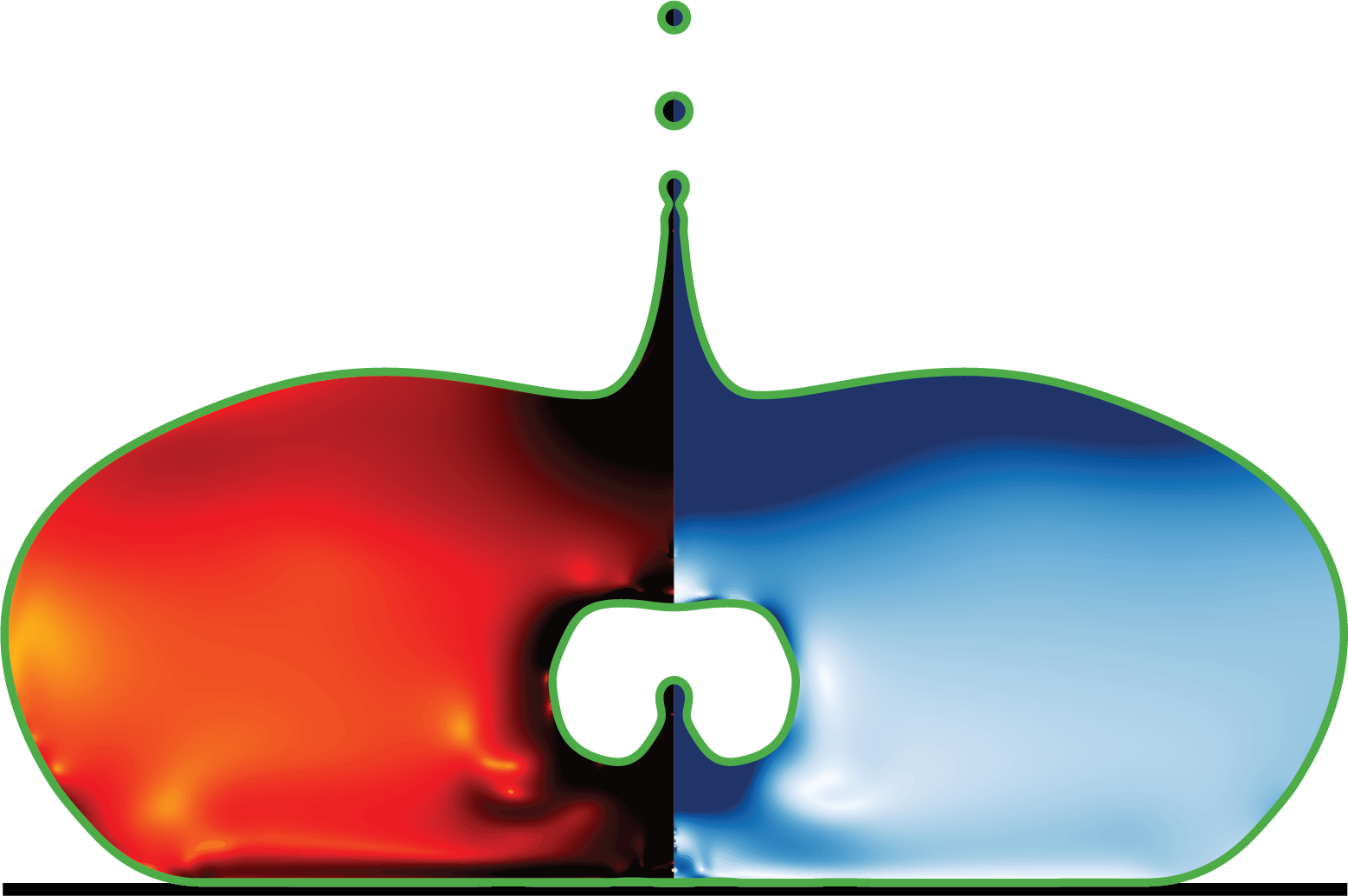
Bursting Bubbles in Viscoelastic Media Simulation
This simulation models the dynamics of bursting bubbles in viscoelastic media using the Basilisk framework. It particularly focuses on the formation of Worthington jets and droplets that emerge during the bursting process.
Physics Overview
The simulation implements a two-phase flow model with viscoelastic properties, utilizing the log-conformation approach for numerical stability. This approach preserves the positive-definiteness of the conformation tensor, which is crucial for stable simulations of viscoelastic fluids at high Deborah numbers.
For theoretical details, see: V. Sanjay, Zenodo, DOI: 10.5281/zenodo.14210635 (2024)
Usage
./program maxLevel De Ec Oh Bond tmaxWhere: - maxLevel: Maximum refinement
level for adaptive mesh - De: Deborah
number (ratio of relaxation time to flow time) -
Ec: Elasto-capillary number (ratio of
elastic to surface tension forces) - Oh:
Ohnesorge number (ratio of viscous to inertial-capillary
forces) - Bond: Bond number (ratio of
gravitational to surface tension forces) -
tmax: Maximum simulation time
@file burstingBubbleVE.c @author Vatsal Sanjay and Ayush Dixit @version 1.0 @date Nov 23, 2024 - Work used in the paper: DOI: 10.1017/jfm.2025.237
#include "axi.h"
#include "navier-stokes/centered.h"

// Uncomment to use the scalar version of the viscoelastic code
// #define _SCALAR

#if !_SCALAR
#include "log-conform-viscoelastic.h"
#else
#include "log-conform-viscoelastic-scalar-2D.h"
#endif
Simulation Parameters
FILTERED: Enable density and viscosity jump smoothingtsnap: Time interval between snapshots (default: 1e-2)fErr: Error tolerance for volume fraction (1e-3)KErr: Error tolerance for curvature calculation (1e-6)VelErr: Error tolerance for velocity field (1e-3)AErr: Error tolerance for conformation tensor (1e-3)Ldomain: Domain size in characteristic lengths (8)
#define FILTERED // Smear density and viscosity jumps
#include "two-phaseVE.h"
#include "navier-stokes/conserving.h"
#include "tension.h"
#if !_MPI
#include "distance.h"
#endif
#define tsnap (1e-2) // 0.001 only for some cases.
// Error tolerances
#define fErr (1e-3) // Error tolerance in f1 VOF
#define KErr (1e-6) // Error tolerance in VoF curvature calculated using height function method
#define VelErr (1e-3) // Error tolerances in velocity - Use 1e-2 for low Oh and 1e-3 to 5e-3 for high Oh/moderate to high J
#define AErr (1e-3) // Error tolerances in conformation inside the liquid
// Domain size
#define Ldomain 8
79
// Boundary conditions - outflow on the right boundary
u.n[right] = neumann(0.);
p[right] = dirichlet(0.);
int MAXlevel;
// Physical parameters:
// Oh -> Solvent Ohnesorge number
// Oha -> air Ohnesorge number
// De -> Deborah number
// Ec -> Elasto-capillary number
double Oh, Oha, De, Ec, Bond, tmax;
char nameOut[80], dumpFile[80];Main Function
Initializes the simulation parameters and sets up the domain.
- Uses command line arguments to set simulation parameters
- Sets up the physical domain with appropriate dimensions
- Configures fluid properties for both phases
- Creates necessary directories for output
int main(int argc, char const *argv[]) {
  dtmax = 1e-5; // BEWARE of this for stability issues.

  L0 = Ldomain;
  origin(-L0/2., 0.);

  // Values taken from the terminal. Here we use some representative values.
  // In production run, you can pass it from the command line.
  MAXlevel = 10; // atoi(argv[1]);
  De = 0.1;      // atof(argv[2]); // Use 1e30 to simulate the De → ∞ limit
  Ec = 0.01;     // atof(argv[3]);
  Oh = 1e-2;     // atof(argv[4]);
  Bond = 1e-3;   // atof(argv[5]);
  tmax = 1e0;    // atof(argv[6]);

  // Ensure that all the variables were transferred properly from the terminal or job script.
  // if (argc < 7){
  //   fprintf(ferr, "Lack of command line arguments. Check! Need %d more arguments\n", 7-argc);
  //   return 1;
  // }

  init_grid(1 << 5);

  // Create a folder named intermediate where all the simulation snapshots are stored.
  char comm[80];
  sprintf(comm, "mkdir -p intermediate");
  system(comm);

  // Name of the restart file. See writingFiles event.
  sprintf(dumpFile, "restart");
Physical Properties Configuration
Sets up the material properties for both phases: -
rho1, rho2: Density of liquid
and gas phases - mu1, mu2:
Dynamic viscosity of liquid and gas phases -
lambda1, lambda2: Relaxation
times - G1, G2: Elastic
moduli
Dimensionless parameters: - Oh:
Ohnesorge number for liquid phase - Oha:
Ohnesorge number for gas phase (= 2e-2 * Oh) -
De: Deborah number - Ec:
Elasto-capillary number - Bond: Bond
number
  rho1 = 1., rho2 = 1e-3;
  Oha = 2e-2 * Oh;
  mu1 = Oh, mu2 = Oha;
  lambda1 = De; lambda2 = 0.;
  G1 = Ec; G2 = 0.;

  f.sigma = 1.0;

  TOLERANCE = 1e-4;
  CFL = 1e-1;

  run();
}
Initialization Event
Sets up the initial conditions for the simulation.
The function attempts to restore from a dump file first. If that fails: - For MPI runs: Ends with an error - For non-MPI runs: Tries to load an initial shape from a data file, creates a distance field, and initializes the volume fraction
event init(t = 0) {
#if _MPI // This is for supercomputers without OpenMP support
  if (!restore(file = dumpFile)) {
    fprintf(ferr, "Cannot restored from a dump file!\n");
  }
#else  // Note that distance.h is incompatible with OpenMPI. So, the below code should not be used with MPI
  if (!restore(file = dumpFile)) {
    char filename[60];
    sprintf(filename, "Bo%5.4f.dat", Bond);
    FILE *fp = fopen(filename, "rb");
    if (fp == NULL) {
      fprintf(ferr, "There is no file named %s\n", filename);
      // Try in folder one level up
      sprintf(filename, "../Bo%5.4f.dat", Bond);
      fp = fopen(filename, "rb");
      if (fp == NULL) {
        fprintf(ferr, "There is no file named %s\n", filename);
        return 1;
      }
    }
    coord *InitialShape;
    InitialShape = input_xy(fp);
    fclose(fp);
    scalar d[];
    distance(d, InitialShape);

    while (adapt_wavelet((scalar *){f, d}, (double[]){1e-8, 1e-8}, MAXlevel).nf);

    // The distance function is defined at the center of each cell, we have
    // to calculate the value of this function at each vertex.
    vertex scalar phi[];
    foreach_vertex() {
      phi[] = -(d[] + d[-1] + d[0,-1] + d[-1,-1])/4.;
    }

    // We can now initialize the volume fraction of the domain.
    fractions(phi, f);
  }
  // return 1;
#endif
}
Adaptive Mesh Refinement
Refines the mesh based on gradients of key fields: - Volume fraction - Velocity components - Conformation tensor components - Curvature
The refinement criteria are set by the error tolerance parameters defined at the beginning of the file. This adaptive approach allows for high resolution in regions of interest while maintaining computational efficiency.
event adapt(i++) {
  scalar KAPPA[];
  curvature(f, KAPPA);

#if !_SCALAR
  adapt_wavelet((scalar *){f, u.x, u.y, conform_p.x.x, conform_p.y.y, conform_p.y.x, conform_qq, KAPPA},
    (double[]){fErr, VelErr, VelErr, AErr, AErr, AErr, AErr, KErr},
    MAXlevel, MAXlevel-6);
#else
  adapt_wavelet((scalar *){f, u.x, u.y, A11, A22, A12, AThTh, KAPPA},
    (double[]){fErr, VelErr, VelErr, AErr, AErr, AErr, AErr, KErr},
    MAXlevel, MAXlevel-6);
#endif
}
Output Management
Creates periodic snapshots of the simulation state. -
Dumps restart files for simulation recovery - Saves
intermediate snapshots at regular intervals defined by
tsnap
event writingFiles(t = 0; t += tsnap; t <= tmax) {
  dump(file = dumpFile);
  sprintf(nameOut, "intermediate/snapshot-%5.4f", t);
  dump(file = nameOut);
}
Simulation Termination
Writes a final summary of the simulation parameters when the simulation ends.
event end(t = end) {
  if (pid() == 0)
    fprintf(ferr, "Level %d, De %2.1e, Ec %2.1e, Oh %2.1e, Oha %2.1e, Bo %4.3f\n",
            MAXlevel, De, Ec, Oh, Oha, Bond);
}
Simulation Logging
Records key simulation data at each timestep: - Iteration number - Timestep size - Current simulation time - Kinetic energy
Also performs safety checks: - Monitors kinetic energy for stability - Terminates simulation if energy becomes too high or too low - Creates log files for post-processing analysis
event logWriting(i++) {
  // Calculate kinetic energy
  double ke = 0.;
  foreach(reduction(+:ke)) {
    ke += (2*pi*y)*(0.5*rho(f[])*(sq(u.x[]) + sq(u.y[])))*sq(Delta);
  }

  if (pid() == 0) {
    static FILE *fp;
    if (i == 0) {
      fprintf(ferr, "Level %d, De %2.1e, Ec %2.1e, Oh %2.1e, Oha %2.1e, Bo %4.3f\n",
              MAXlevel, De, Ec, Oh, Oha, Bond);
      fprintf(ferr, "De Ec Oh i dt t ke\n");
      fp = fopen("log", "w");
      fprintf(fp, "Level %d, De %2.1e, Ec %2.1e, Oh %2.1e, Oha %2.1e, Bo %4.3f\n",
              MAXlevel, De, Ec, Oh, Oha, Bond);
      fprintf(fp, "i dt t ke\n");
      fprintf(fp, "%d %g %g %g\n", i, dt, t, ke);
      fclose(fp);
    } else {
      fp = fopen("log", "a");
      fprintf(fp, "%d %g %g %g\n", i, dt, t, ke);
      fclose(fp);
    }
    fprintf(ferr, "%d %g %g %g\n", i, dt, t, ke);

    assert(ke > -1e-10);

    // Check for energy blowup (numerical instability)
    if (ke > 1e2 && i > 1e1) {
      if (pid() == 0) {
        fprintf(ferr, "The kinetic energy blew up. Stopping simulation\n");
        fp = fopen("log", "a");
        fprintf(fp, "The kinetic energy blew up. Stopping simulation\n");
        fclose(fp);
        dump(file = dumpFile);
        return 1;
      }
    }
    assert(ke < 1e2);

    // Check for energy dissipation below threshold
    if (ke < 1e-6 && i > 1e1) {
      if (pid() == 0) {
        fprintf(ferr, "kinetic energy too small now! Stopping!\n");
        dump(file = dumpFile);
        fp = fopen("log", "a");
        fprintf(fp, "kinetic energy too small now! Stopping!\n");
        fclose(fp);
        return 1;
      }
    }
  }
}