
CoMPhy Lab · Research snapshot
Darwin drift past fixed obstacles
How much fluid does an obstacle carry with it? We compute the permanent drift of material lines past a sphere, a circular cylinder and a patch of 25 cylinders in steady viscous flow, and compare it with the classical potential-flow and Stokes-flow limits.
Snapshot of results, October 2026. Work in progress; values may be refined.
In brief
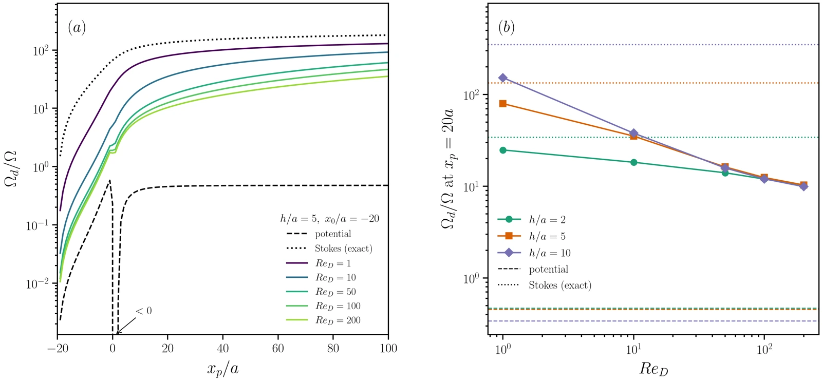
- In ideal (potential) flow the drift equals the obstacle's added-mass volume: half its own volume for a sphere, and the area of its circular cross-section, πa², for a cylinder. In viscous flow the drift is far larger. For a marked sheet released 20 radii upstream and observed 20 radii downstream, 2 to 10 radii in half-width, it is 10 to 150 times the obstacle's volume (sphere) or area (cylinder) at Reynolds numbers 1 to 200, against less than one for potential flow.
- At that plane the viscous drift falls steadily with Reynolds number, and every viscous curve keeps growing the further downstream it is measured. The drift is therefore a map over measurement windows, not a single number.
- Thirty radii behind a 25-cylinder patch at solid fraction 0.1 (ReD = 1 and 2), the drift is about 570 to 770 single-cylinder areas, including fluid held in the patch's standing eddies. A random layout and a 5×5 lattice with the same number of cylinders differ by at most about 2%, and by how much depends on how the two layouts are aligned, so no effect of arrangement is resolved yet.
- The drift measurement reproduces exact potential-flow and Stokes-flow results, and the flow solutions reproduce published drag, wake and instability data.
The question
When a body moves through fluid, it carries fluid with it. A sheet of marked fluid that the body passes through is left permanently bent, and the volume between the bent sheet and its starting position is the drift volume Ωd. For a body moving through unbounded ideal fluid, Darwin (1953) showed that the drift equals the added-mass volume: half the volume for a sphere and the area of its circular cross-section, πa², for a cylinder. The equality holds only when the path of the body is much longer than the sheet is wide. A sheet released a finite distance from the body gives instead the "partial drift" (Eames, Belcher & Hunt 1994), whose value depends on the ratio of the sheet's width to that distance.
Viscous flow changes the picture. In Stokes flow the disturbance decays only as 1/r, and the drift of an unbounded sheet is infinite (Eames, Gobby & Dalziel 2003; Chisholm & Khair 2017). At finite Reynolds number the wake carries a volume deficit set by the drag, so the drift keeps growing downstream. We therefore measure the drift in a stated window and report it as Ωd/Ω, where Ω is the volume or area of one obstacle.
How each result is produced
- Steady flowFinite elements with Taylor–Hood (P2/P1) triangles in pyoomph, Newton's method with continuation in Reynolds number. The sphere is axisymmetric; the cylinder and patch are planar.
- SteadinessLinear stability by shift-and-invert eigenvalue searches around complex shifts, covering the wake-shedding frequencies.
- Field evaluationDirect evaluation of the quadratic finite-element velocity, with a persistent point locator.
- DriftBounding streamlines released by label and traced with an embedded Runge–Kutta scheme; the tube volume follows from contour integrals.
- OutputDrift maps over the observation plane and aperture, and material lines traced through each steady flow.
Results: sphere and cylinder

| Flow | Sphere | Cylinder | ||||
|---|---|---|---|---|---|---|
| h = 2a | h = 5a | h = 10a | h = 2a | h = 5a | h = 10a | |
| Potential (exact) | 0.47 | 0.45 | 0.34 | 0.78 | 0.67 | 0.40 |
| Stokes, unbounded (exact) | 34.2 | 133.4 | 349.0 | – | – | – |
| ReD = 1 | 24.9 | 79.6 | 152.7 | 36.2 | 57.4 | 69.2 |
| ReD = 2 | – | – | – | 30.5 | 44.7 | 49.6 |
| ReD = 5 | – | – | – | 24.7 | 31.3 | 30.9 |
| ReD = 10 | 18.3 | 35.2 | 37.9 | 21.7 | 24.6 | 23.2 |
| ReD = 20 | – | – | – | 19.4 | 20.0 | 18.4 |
| ReD = 40 | – | – | – | 18.0 | 17.5 | 15.9 |
| ReD = 50 | 14.0 | 16.2 | 15.8 | – | – | – |
| ReD = 100 | 12.0 | 12.4 | 12.0 | – | – | – |
| ReD = 200 | 10.3 | 10.3 | 9.9 | – | – | – |
- Measured At ReD = 1 to 200, viscous drift is 10–150 obstacle volumes (sphere) or areas (cylinder) in these windows, rising to 34–349 sphere volumes in exact Stokes flow, against 0.3–0.8 for potential flow in the same windows. The potential values lie below Darwin's ½ and 1 because the windows are finite.
- Measured At xp = 20a the drift falls steadily with Reynolds number: at h = 5a, from 80 to 10 for the sphere (ReD 1 to 200) and from 57 to 17 for the cylinder (ReD 1 to 40). No viscous curve levels off; all are still rising at xp = 100a.
- Measured The aperture matters strongly at low Reynolds number and much less at high. For the sphere at ReD = 1, apertures of 2a, 5a and 10a give 25, 80 and 153; at ReD = 200 they give 10.3, 10.3 and 9.9.
- Interpretation This fits a drift carried by the wake's volume deficit. The drag sets that deficit, so while the wake lies inside the window the drift grows downstream at a rate proportional to the drag (Chisholm & Khair 2017). At low Reynolds number the disturbance is broad, so a wider sheet collects more lag; at high Reynolds number the deficit sits in a thin wake that even the narrowest window encloses.
- Measured Where the flow recirculates (the sphere from ReD = 50, the cylinder from 10), the drift includes the fluid held in the standing eddy behind the body, which no material line enters.
- Measured The computed Stokes flow past the sphere (not shown in the figure) gives drift 3.6–16.7% below the exact unbounded solution. On a small verification domain with the exact solution imposed on its boundary, the drift error on the finest mesh falls to about 10−6 sphere volumes, so the difference reflects the finite computational domain: Stokes flow decays so slowly that the outer boundary matters. At ReD = 1 the domain effect is estimated at 1–2%.
Results: 25-cylinder patch

| Aperture h | ReD = 1 | ReD = 2 | ||||
|---|---|---|---|---|---|---|
| lattice | random | difference | lattice | random | difference | |
| 14.0a (Lp/2) | 770.2 | 755.0 | −2.0% | 707.3 | 693.9 | −1.9% |
| 21.0a | 753.4 | 739.1 | −1.9% | 678.2 | 665.9 | −1.8% |
| 28.0a | 722.9 | 709.5 | −1.8% | 643.3 | 632.1 | −1.7% |
| 42.0a | 653.7 | 641.9 | −1.8% | 576.2 | 566.6 | −1.7% |
- Measured Thirty radii behind the nominal patch outline, the drift is about 570–770 single-cylinder areas, depending on the window and the Reynolds number. At both Reynolds numbers the value includes fluid held in the patch's standing eddies. At ReD = 1 the eddies close near x ≈ 30a, upstream of this plane, so all of their fluid is counted; at ReD = 2 this plane cuts through them. The material that passes the patch lags by less.
- Measured At a fixed plane the drift falls as the window widens. In the videos the outer part of the line runs ahead of its no-body position.
- Interpretation The wide windows include fluid pushed sideways around the patch, which moves faster than the free stream.
- Measured The lateral boundaries of the computational domain lower the patch drift slightly: widening the domain by half raises it by 0.9–2.8% at xp = 44a, by the same factor for both layouts. Mesh refinement changes the drift by at most 0.02%.
- Measured With the same planes for both layouts, the random layout drifts 1.7–2.0% less than the lattice at xp = 44a. The random layout's cylinders, however, extend 1.6a further downstream than the lattice's, and with each window placed at the same distances from each layout's rear edge the difference falls to 0.1–0.5%.
- Interpretation The difference depends on how the layouts are aligned, and it comes from a single random layout. No effect of arrangement is resolved yet.
- Measured Both patches carry a patch-scale pair of standing eddies. At ReD = 2 their rear stagnation point lies at x ≈ 54a from the patch centre, about 40a (1.4Lp) behind the patch. The material line stays caught at the front cylinders long after the outer line has passed: little fluid flows through the patch.
- Interpretation At this solid fraction and these Reynolds numbers the patch behaves much like one porous bluff body (compare Nicolle & Eames 2011). Its least-damped linear mode at ReD = 2 oscillates with a Strouhal number of about 0.115 based on the patch width, close to the value for a single cylinder at the onset of vortex shedding (0.117, table below); that mode is still damped.
Material lines in the steady flows
Each video holds the flow fixed at its converged steady state and follows a material line released at x₀ = −15a with aperture h = 5a for the sphere and cylinder (the drift figures above use x₀ = −20a), and at x₀ = −24.0a with h = 21.0a for the patch. All six flows are steady (see the steadiness table below).
Verification and validation
| Check | Result | Reference |
|---|---|---|
| Displacement of fluid particles after complete passage, exact potential flow past a cylinder | agrees with Darwin's closed-form expression to 10−10 | Darwin (1953) |
| Streamtube drift, exact Stokes flow past a sphere, window x₀ = −2h, xp = 2h | relative error below 10−9 against independent quadrature; Dst/a³ = 1461.967 (h = 10a) and 389.859 (h = 5a) | exact Stokes flow; drift definition of Chisholm & Khair (2017) |
| Computed Stokes sphere on a small domain with exact boundary values, three meshes | drift error 3.9×10⁻⁴, 1.2×10⁻⁴, 1.2×10⁻⁶ Ω | exact Stokes flow |
| Sphere drag, ReD = 100, 200 | within about 0.04% on the reference's truncated domain; 0.14–0.15% lower in the larger production domain | Tabata & Itakura (1998) |
| Sphere, onset of separation | between ReD = 20 and 20.5 | 20.5, Dennis & Walker (1971) |
| Cylinder drag, ReD = 10, 40 | CD = 2.790 (−0.18%), 1.509 (−0.01%) | Sen, Mittal & Biswas (2009); at ReD = 10, from their fitted correlation |
| Cylinder wake, ReD = 40 | length 2.249D, separation angle 53.60° | Sen, Mittal & Biswas (2009) |
| Cylinder, onset of vortex shedding | ReD = 46.71–46.72, Strouhal number 0.1167 | 46.7 to 47.4 in Giannetti & Luchini (2007) and Kumar & Mittal (2006) |
| Patch, mesh convergence | relative drift change at most 2×10⁻⁴ (0.02%) between the two finest meshes | three meshes |
| Patch, lateral domain enlarged by half | drift +0.9% to +2.8% at xp = 44a, the same factor for both layouts | two domains |
| State | Growth rate | Angular frequency | Verdict |
|---|---|---|---|
| Cylinder, ReD = 10 | −0.0396 | 0.017 | stable within the searched region |
| Cylinder, ReD = 20 | −0.0412 | 0.016 | stable within the searched region |
| Cylinder, ReD = 40 | −0.0310 | 0.720 | stable within the searched region (wake mode) |
| Patch, random and lattice, ReD = 1 | −0.0131 | 0 | stable within the searched region |
| Patch, random and lattice, ReD = 2 | −0.0073, −0.0074 | 0.052, 0.051 | stable within the searched region |
| Sphere, ReD = 200 (least-stable of the axisymmetric and first non-axisymmetric modes at 100 and 200) | −0.0374 | 0 | stable within the searched region, on reduced domains (not the drift domains) |
For the cylinder and the patch, "stable within the searched region" means a regional eigenvalue search on a coarser mesh followed by confirmation of the leading mode on the production mesh. For the sphere, the search was repeated on two meshes in two computational domains smaller than the one used for the drift. It is a numerical assessment, not a proof that no unstable mode exists elsewhere in the spectrum. The sphere at ReD ≤ 50 and the cylinder at ReD ≤ 5 were not assessed; they lie far below the known instabilities of these flows.
Limitations of this snapshot
- Only steady flows are computed, all in finite domains. The domain shifts the drift by about 1–3% for the patch, and by up to 17% for the sphere in Stokes flow, falling to an estimated 1–2% at ReD = 1. The sensitivity of the single-cylinder drift to the lateral boundaries has not been measured, and the cylinder runs use a lateral half-width of 150a for ReD ≤ 2 and 100a for ReD ≥ 5.
- Where the flow recirculates, the drift includes fluid trapped in standing eddies; this volume has not yet been separated from the drift of the material that passes the obstacles.
- The arrangement comparison rests on a single random layout and depends on how the layouts are aligned.
- Stability is assessed within a searched region of the spectrum, not globally. The sphere flows at ReD = 100 and 200 were tested only on reduced computational domains; ReD = 200 lies just below the non-axisymmetric instability at ReD ≈ 210 (Natarajan & Acrivos 1993).
- The computed onset of cylinder vortex shedding, 46.71, lies at the lower end of published linear-stability values.
Methods, software and references
Flows were computed with pyoomph (Diddens & Rocha 2024), built on oomph-lib (Heil & Hazel 2006), using the CoMPhy fork comphy-lab/pyoomph at commit f912ac10, with Taylor–Hood elements (Taylor & Hood 1973), Gmsh meshes (Geuzaine & Remacle 2009) and the Spectra shift-and-invert eigensolver with Pardiso and SuperLU sparse factorisations. The drift measurement and figures were produced with the comphy-lab/darwin-drift solver; the figures at commit c5f8b18.
- Chisholm, N. G. & Khair, A. S. 2017 Drift volume in viscous flows. Phys. Rev. Fluids 2, 064101. doi:10.1103/PhysRevFluids.2.064101
- Darwin, C. 1953 Note on hydrodynamics. Proc. Camb. Phil. Soc. 49, 342–354. doi:10.1017/S0305004100028449
- Dennis, S. C. R. & Walker, J. D. A. 1971 Calculation of the steady flow past a sphere at low and moderate Reynolds numbers. J. Fluid Mech. 48, 771–789. doi:10.1017/S0022112071001848
- Diddens, C. & Rocha, D. 2024 Bifurcation tracking on moving meshes and with consideration of azimuthal symmetry breaking instabilities. J. Comput. Phys. 518, 113306. doi:10.1016/j.jcp.2024.113306
- Eames, I., Belcher, S. E. & Hunt, J. C. R. 1994 Drift, partial drift and Darwin's proposition. J. Fluid Mech. 275, 201–223. doi:10.1017/S0022112094002338
- Eames, I., Gobby, D. & Dalziel, S. B. 2003 Fluid displacement by Stokes flow past a spherical droplet. J. Fluid Mech. 485, 67–85. doi:10.1017/S0022112003004361
- Geuzaine, C. & Remacle, J.-F. 2009 Gmsh: a 3-D finite element mesh generator with built-in pre- and post-processing facilities. Int. J. Numer. Meth. Engng 79, 1309–1331. doi:10.1002/nme.2579
- Giannetti, F. & Luchini, P. 2007 Structural sensitivity of the first instability of the cylinder wake. J. Fluid Mech. 581, 167–197. doi:10.1017/S0022112007005654
- Heil, M. & Hazel, A. L. 2006 oomph-lib — an object-oriented multi-physics finite-element library. In Fluid-Structure Interaction, Lecture Notes in Computational Science and Engineering 53, 19–49. Springer. doi:10.1007/3-540-34596-5_2
- Kumar, B. & Mittal, S. 2006 Effect of blockage on critical parameters for flow past a circular cylinder. Int. J. Numer. Meth. Fluids 50, 987–1001. doi:10.1002/fld.1098
- Natarajan, R. & Acrivos, A. 1993 The instability of the steady flow past spheres and disks. J. Fluid Mech. 254, 323–344. doi:10.1017/S0022112093002150
- Nicolle, A. & Eames, I. 2011 Numerical study of flow through and around a circular array of cylinders. J. Fluid Mech. 679, 1–31. doi:10.1017/jfm.2011.77
- Sen, S., Mittal, S. & Biswas, G. 2009 Steady separated flow past a circular cylinder at low Reynolds numbers. J. Fluid Mech. 620, 89–119. doi:10.1017/S0022112008004904
- Tabata, M. & Itakura, K. 1998 A precise computation of drag coefficients of a sphere. Int. J. Comput. Fluid Dyn. 9, 303–311. doi:10.1080/10618569808940861
- Taylor, C. & Hood, P. 1973 A numerical solution of the Navier–Stokes equations using the finite element technique. Comput. Fluids 1, 73–100. doi:10.1016/0045-7930(73)90027-3