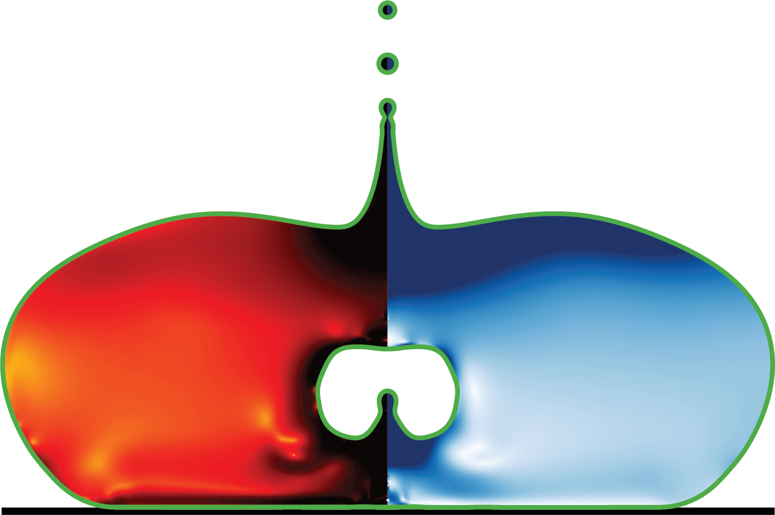
postProcess/Video-generic.py
#!/usr/bin/env python3
# -*- coding: utf-8 -*-
Basilisk Fluid Dynamics Visualization Script
This script processes Basilisk simulation snapshots to create high-quality visualizations of fluid dynamics simulations, particularly for soap bubble and multiphase flow problems. It reads simulation data from intermediate snapshot files, extracts facet information (interfaces), and temperature/scalar fields, then generates publication-quality plots.
The script supports parallel processing for efficient generation of animation frames from large simulation datasets.
Usage: python Video-generic.py [options]
Basic usage: python Video-generic.py -CPUs 8 -nGFS 1000
Custom simulation: python Video-generic.py -caseToProcess ../mySimulation -RMAX 5.0
Dependencies: - numpy: For numerical operations - matplotlib: For visualization - multiprocessing: For parallel processing - subprocess: For calling external Basilisk utilities - argparse: For command-line argument parsing
External Requirements: - ./getFacet: Basilisk utility to extract interface facets - ./getData: Basilisk utility to extract field data - LaTeX: For rendering mathematical expressions in plots
Author: Vatsal Sanjay Email: [email protected] Affiliation: CoMPhy Lab, Physics of Fluids Department Last updated: Mar 8, 2025
import numpy as np
import os
import subprocess as sp
import matplotlib
import matplotlib.pyplot as plt
from matplotlib.collections import LineCollection
from matplotlib.ticker import StrMethodFormatter
import multiprocessing as mp
from functools import partial
import argparse
import sys

# ===============================
# Matplotlib Configuration
# ===============================
matplotlib.rcParams['font.family'] = 'serif'
matplotlib.rcParams['text.usetex'] = True
matplotlib.rcParams['text.latex.preamble'] = r'\usepackage{amsmath}'

# ===============================
# Data Extraction Functions
# ===============================

def gettingFacets(filename, includeCoat='true'):
Extract interface facets from a Basilisk snapshot file.
This function calls the external getFacet utility to extract the coordinates of interface segments (facets) from a Basilisk simulation snapshot. The facets represent the boundaries between different phases or the free surface.
The function automatically mirrors facets across the r=0 axis for axisymmetric simulations, creating a full 2D representation.
Args: filename (str): Path to the Basilisk snapshot file includeCoat (str, optional): Whether to include coating interfaces. Defaults to ‘true’.
Returns: list: List of line segments, where each segment is a tuple of two points ((r1, z1), (r2, z2)). Returns empty list if file has insufficient data.
Raises: subprocess.CalledProcessError: If getFacet utility fails
Example: >>> facets = gettingFacets(“snapshot-0.1000”) >>> print(f”Found {len(facets)} facet segments”)
    # Execute the getFacet utility
    exe = ["./getFacet", filename, includeCoat]
    p = sp.Popen(exe, stdout=sp.PIPE, stderr=sp.PIPE)
    stdout, stderr = p.communicate()

    # Parse the output from stderr (Basilisk utilities output to stderr)
    temp1 = stderr.decode("utf-8")
    temp2 = temp1.split("\n")
    segs = []
    skip = False

    # Only process if we have substantial output (>100 lines indicates valid data)
    if (len(temp2) > 1e2):
        for n1 in range(len(temp2)):
            temp3 = temp2[n1].split(" ")
            if temp3 == ['']:
                skip = False
                pass
            else:
                if not skip:
                    # Parse the next line for the second point of the segment
                    temp4 = temp2[n1+1].split(" ")
                    # Note: getFacet outputs in (z, r) format, we convert to (r, z)
                    r1, z1 = np.array([float(temp3[1]), float(temp3[0])])
                    r2, z2 = np.array([float(temp4[1]), float(temp4[0])])

                    # Add the original segment
                    segs.append(((r1, z1), (r2, z2)))
                    # Mirror across r=0 for axisymmetric visualization
                    segs.append(((-r1, z1), (-r2, z2)))
                    skip = True

    return segs


def gettingfield(filename, zmin, zmax, rmax, nr):
Extract field data from a Basilisk snapshot within specified bounds.
This function calls the getData utility to extract scalar field data (e.g., temperature, concentration) from a Basilisk simulation on a regular grid. The data is extracted in a rectangular region for efficient visualization.
Args: filename (str): Path to the Basilisk snapshot file zmin (float): Minimum z-coordinate for data extraction zmax (float): Maximum z-coordinate for data extraction rmax (float): Maximum radial coordinate for data extraction nr (int): Number of grid points in the radial direction
Returns: tuple: Contains: - R (numpy.ndarray): 2D array of radial coordinates (nz x nr) - Z (numpy.ndarray): 2D array of axial coordinates (nz x nr) - T (numpy.ndarray): 2D array of field values (nz x nr) - nz (int): Number of grid points in the axial direction
Raises: subprocess.CalledProcessError: If getData utility fails ValueError: If data reshaping fails due to inconsistent dimensions
Example: >>> R, Z, T, nz = gettingfield(“snapshot-0.1000”, 0, 4, 2, 256) >>> print(f”Grid size: {nz} x {nr}“)
    # Execute the getData utility with specified bounds
    exe = ["./getData", filename, str(zmin), str(0), str(zmax), str(rmax), str(nr)]
    p = sp.Popen(exe, stdout=sp.PIPE, stderr=sp.PIPE)
    stdout, stderr = p.communicate()

    # Parse the output
    temp1 = stderr.decode("utf-8")
    temp2 = temp1.split("\n")
    Rtemp, Ztemp, Ttemp = [], [], []

    # Extract data points from output
    for n1 in range(len(temp2)):
        temp3 = temp2[n1].split(" ")
        if temp3 == ['']:
            pass
        else:
            # getData outputs in (z, r, field) format
            Ztemp.append(float(temp3[0]))
            Rtemp.append(float(temp3[1]))
            Ttemp.append(float(temp3[2]))

    # Convert to numpy arrays
    R = np.asarray(Rtemp)
    Z = np.asarray(Ztemp)
    T = np.asarray(Ttemp)

    # Calculate grid dimensions
    nz = int(len(Z)/nr)
    print("nz is %d" % nz)

    # Reshape into 2D grids for visualization
    R.resize((nz, nr))
    Z.resize((nz, nr))
    T.resize((nz, nr))

    return R, Z, T, nz


# ===============================
# Visualization Functions
# ===============================

def process_timestep(ti, caseToProcess, folder, tsnap, GridsPerR, rmin, rmax, zmin, zmax, lw):
Process and visualize a single timestep from the simulation.
This function handles the complete visualization pipeline for one timestep: reading data, creating the plot with field visualization and interface contours, and saving the image. It’s designed to be called in parallel for multiple timesteps.
The visualization includes: - Temperature/scalar field as a colored heatmap - Interface facets as blue lines - Domain boundaries - Axis of symmetry (for axisymmetric cases)
Args: ti (int): Timestep index caseToProcess (str): Path to the simulation case directory folder (str): Output directory for saving images tsnap (float): Time interval between snapshots GridsPerR (int): Number of grid points per unit radius rmin (float): Minimum radial coordinate for plotting rmax (float): Maximum radial coordinate for plotting zmin (float): Minimum axial coordinate for plotting zmax (float): Maximum axial coordinate for plotting lw (float): Line width for plotting boundaries
Returns: None: Saves image to disk
Note: - Skips processing if output image already exists - Prints error messages if snapshot file is missing or corrupted - Images are saved with 8-digit zero-padded filenames for proper sorting
Example: >>> process_timestep(100, “../simCase”, “output”, 0.01, 128, -2, 2, 0, 4, 2) # Creates output/00001000.png for t=1.0
    # Calculate physical time for this timestep
    t = tsnap * ti
    place = f"{caseToProcess}/intermediate/snapshot-{t:.4f}"
    name = f"{folder}/{int(t*1000):08d}.png"

    # Check if snapshot file exists
    if not os.path.exists(place):
        print(f"{place} File not found!")
        return

    # Skip if output already exists (useful for resuming interrupted runs)
    if os.path.exists(name):
        print(f"{name} Image present!")
        return

    # Extract interface facets
    segs = gettingFacets(place)

    if not segs:
        print(f"Problem in the available file {place}")
        return

    # Calculate grid resolution based on domain size
    nr = int(GridsPerR * rmax)

    # Extract field data
    R, Z, T, nz = gettingfield(place, zmin, zmax, rmax, nr)
    zminp, zmaxp, rminp, rmaxp = Z.min(), Z.max(), R.min(), R.max()

    # ===============================
    # Plotting Configuration
    # ===============================
    AxesLabel, TickLabel = 50, 20
    fig, ax = plt.subplots()
    fig.set_size_inches(19.20, 10.80)  # Full HD resolution

    # Plot domain boundaries and axis of symmetry
    ax.plot([0, 0], [zmin, zmax], '-.', color='grey', linewidth=lw)  # Symmetry axis
    ax.plot([rmin, rmin], [zmin, zmax], '-', color='black', linewidth=lw)  # Left boundary
    ax.plot([rmin, rmax], [zmin, zmin], '-', color='black', linewidth=lw)  # Bottom boundary
    ax.plot([rmin, rmax], [zmax, zmax], '-', color='black', linewidth=lw)  # Top boundary
    ax.plot([rmax, rmax], [zmin, zmax], '-', color='black', linewidth=lw)  # Right boundary

    # Add interface facets as a collection for efficiency
    line_segments = LineCollection(segs, linewidths=4, colors='blue', linestyle='solid')
    ax.add_collection(line_segments)

    # Create temperature/scalar field visualization
    cntrl2 = ax.imshow(T, interpolation='Bilinear', cmap='hot_r', origin='lower',
                       extent=[rminp, rmaxp, zminp, zmaxp], vmax=1.0, vmin=0.0)

    # Configure plot appearance
    ax.set_aspect('equal')
    ax.set_xlim(rmin, rmax)
    ax.set_ylim(zmin, zmax)
    ax.set_title(f'$t/\\tau_\\gamma$ = {t:4.3f}', fontsize=TickLabel)
    ax.axis('off')  # Remove axes for cleaner visualization

    # Save figure with tight layout
    plt.savefig(name, bbox_inches="tight")
    plt.close()


# ===============================
# Main Execution
# ===============================

def main():
Main function that orchestrates the parallel visualization process.
This function: 1. Parses command-line arguments for configuration 2. Sets up the output directory 3. Creates a multiprocessing pool 4. Distributes timestep processing across available CPUs
The parallel processing significantly speeds up visualization of large simulation datasets by processing multiple timesteps simultaneously.
    parser = argparse.ArgumentParser(
        description='Generate visualizations from Basilisk simulation snapshots',
        formatter_class=argparse.RawDescriptionHelpFormatter)

    parser.add_argument('--CPUs', type=int, default=8,
                       help='Number of CPUs to use for parallel processing')
    parser.add_argument('--nGFS', type=int, default=4000,
                       help='Number of snapshot files to process')
    parser.add_argument('--GridsPerR', type=int, default=128,
                       help='Grid resolution per unit radius (affects image quality)')
    parser.add_argument('--ZMAX', type=float, default=4.0,
                       help='Maximum Z coordinate for visualization domain')
    parser.add_argument('--RMAX', type=float, default=4.0,
                       help='Maximum R coordinate for visualization domain')
    parser.add_argument('--ZMIN', type=float, default=0.0,
                       help='Minimum Z coordinate for visualization domain')
    parser.add_argument('--tsnap', type=float, default=0.01,
                       help='Time interval between snapshots')
    parser.add_argument('--caseToProcess', type=str,
                       default='../simulationCases/soapBubble-full',
                       help='Path to simulation case directory')
    parser.add_argument('--folderToSave', type=str, default='Video',
                       help='Output directory for images')

    args = parser.parse_args()

    # Extract arguments
    num_processes = args.CPUs
    nGFS = args.nGFS
    tsnap = args.tsnap
    ZMAX = args.ZMAX
    RMAX = args.RMAX
    ZMIN = args.ZMIN

    # Set up visualization domain (full domain for axisymmetric cases)
    rmin, rmax, zmin, zmax = [-RMAX, RMAX, ZMIN, ZMAX]
    GridsPerR = args.GridsPerR

    # Visualization parameters
    lw = 2  # Line width for boundaries
    folder = args.folderToSave
    caseToProcess = args.caseToProcess

    # Create output directory if it doesn't exist
    if not os.path.isdir(folder):
        os.makedirs(folder)
        print(f"Created output directory: {folder}")

    # ===============================
    # Parallel Processing
    # ===============================
    print(f"Starting parallel processing with {num_processes} CPUs...")
    print(f"Processing {nGFS} timesteps from {caseToProcess}")

    # Create a pool of worker processes
    with mp.Pool(processes=num_processes) as pool:
        # Create partial function with fixed arguments
        # This allows us to pass only the timestep index to each worker
        process_func = partial(process_timestep,
                             caseToProcess=caseToProcess,
                             folder=folder,
                             tsnap=tsnap,
                             GridsPerR=GridsPerR,
                             rmin=rmin,
                             rmax=rmax,
                             zmin=zmin,
                             zmax=zmax,
                             lw=lw)

        # Map the process function to all timesteps
        # This distributes the work across available CPUs
        pool.map(process_func, range(nGFS))

    print(f"Processing complete! Images saved to {folder}/")
    print("To create a video from images, use:")
    print(f"  ffmpeg -framerate 30 -pattern_type glob -i '{folder}/*.png' -c:v libx264 output.mp4")


if __name__ == "__main__":
    main()