postProcess/VideoAxi.py
#!/usr/bin/env python3
# -*- coding: utf-8 -*-
Viscoelastic Visualization Tool
This script processes and visualizes fluid dynamics simulation data, particularly focused on droplet impact and deformable soft matter like liquid drops, sheets, and bubbles. It extracts interface positions and scalar field data from simulation files and creates visualizations showing physical quantities like strain rates and stresses.
The script is designed to process multiple simulation snapshots in parallel, extracting data using external executables and generating visualizations with proper colormaps, scales, and mathematical labels.
Features: - Extracts fluid interfaces and scalar fields from simulation files - Generates visualizations with proper colormaps and mathematical labels - Processes multiple timesteps in parallel using multiprocessing - Configurable via command-line arguments for different simulation cases - Creates publication-quality figures with LaTeX-rendered mathematical expressions
Usage: python fluid_vis.py [options]
Command-line Arguments: –CPUs Number of CPUs to use for parallel processing (default: all available) –nGFS Number of restart files to process (default: 550) –ZMAX Maximum Z coordinate for visualization (default: 4.0) –RMAX Maximum R coordinate for visualization (default: 2.0) –ZMIN Minimum Z coordinate for visualization (default: -4.0) –caseToProcess Path to simulation case directory (default: ‘../simulationCases/dropImpact’) –folderToSave Directory to save visualization images (default: ‘dropImpact’)
Dependencies: External executables: getFacet2D, getData-elastic-scalar2D Python libraries: numpy, matplotlib, subprocess, multiprocessing
Author: Vatsal Sanjay Email: [email protected] Affiliation: Physics of Fluids Last updated: Jul 24, 2024
import numpy as np
import os
import subprocess as sp
import matplotlib
import matplotlib.pyplot as plt
from matplotlib.collections import LineCollection
from matplotlib.ticker import StrMethodFormatter
import multiprocessing as mp
from functools import partial
import argparse

import matplotlib.colors as mcolors
custom_colors = ["white", "#DA8A67", "#A0522D", "#400000"]
custom_cmap = mcolors.LinearSegmentedColormap.from_list("custom_hot", custom_colors)

# Configure matplotlib for publication-quality figures with LaTeX rendering
matplotlib.rcParams['font.family'] = 'serif'
matplotlib.rcParams['text.usetex'] = True
matplotlib.rcParams['text.latex.preamble'] = r'\usepackage{amsmath}'

def gettingFacets(filename, includeCoat='true'):
Extract interface positions (facets) from simulation files.
Args: filename (str): Path to simulation snapshot file includeCoat (str, optional): Whether to include coating layer. Defaults to ‘true’.
Returns: list: List of line segments defining fluid interfaces
    exe = ["./getFacet2D", filename, includeCoat]
    p = sp.Popen(exe, stdout=sp.PIPE, stderr=sp.PIPE)
    stdout, stderr = p.communicate()
    temp1 = stderr.decode("utf-8")
    temp2 = temp1.split("\n")
    segs = []
    skip = False
    if (len(temp2) > 1e2):
        for n1 in range(len(temp2)):
            temp3 = temp2[n1].split(" ")
            if temp3 == ['']:
                skip = False
                pass
            else:
                if not skip:
                    temp4 = temp2[n1+1].split(" ")
                    r1, z1 = np.array([float(temp3[1]), float(temp3[0])])
                    r2, z2 = np.array([float(temp4[1]), float(temp4[0])])
                    segs.append(((r1, z1),(r2, z2)))
                    segs.append(((-r1, z1),(-r2, z2)))
                    skip = True
    return segs

def gettingfield(filename, zmin, zmax, rmax, nr):
Extract scalar field data from simulation files.
Args: filename (str): Path to simulation snapshot file zmin (float): Minimum Z coordinate zmax (float): Maximum Z coordinate rmax (float): Maximum R coordinate nr (int): Number of grid points in R direction
Returns: tuple: (R, Z, D2, vel, taup, nz) arrays of coordinates and field values
    exe = ["./getData-elastic-scalar2D", filename, str(zmin), str(0), str(zmax), str(rmax), str(nr)]
    p = sp.Popen(exe, stdout=sp.PIPE, stderr=sp.PIPE)
    stdout, stderr = p.communicate()
    temp1 = stderr.decode("utf-8")
    temp2 = temp1.split("\n")
    # print(temp2) #debugging
    Rtemp, Ztemp, D2temp, veltemp, taupTemp  = [],[],[],[],[]

    for n1 in range(len(temp2)):
        temp3 = temp2[n1].split(" ")
        if temp3 == ['']:
            pass
        else:
            Ztemp.append(float(temp3[0]))
            Rtemp.append(float(temp3[1]))
            D2temp.append(float(temp3[2]))
            veltemp.append(float(temp3[3]))
            taupTemp.append(float(temp3[4]))

    R = np.asarray(Rtemp)
    Z = np.asarray(Ztemp)
    D2 = np.asarray(D2temp)
    vel = np.asarray(veltemp)
    taup = np.asarray(taupTemp)
    nz = int(len(Z)/nr)

    # print("nr is %d %d" % (nr, len(R))) # debugging
    print("nz is %d" % nz)

    R.resize((nz, nr))
    Z.resize((nz, nr))
    D2.resize((nz, nr))
    vel.resize((nz, nr))
    taup.resize((nz, nr))

    return R, Z, D2, vel, taup, nz
# ----------------------------------------------------------------------------------------------------------------------

def process_timestep(ti, folder, nGFS, GridsPerR, rmin, rmax, zmin, zmax, lw, caseToProcess):
Process a single timestep from simulation data and generate visualization.
Args: ti (int): Timestep index folder (str): Directory to save output images nGFS (int): Total number of timesteps GridsPerR (int): Grid points per unit length in R direction rmin (float): Minimum R coordinate rmax (float): Maximum R coordinate zmin (float): Minimum Z coordinate zmax (float): Maximum Z coordinate lw (float): Line width for plot elements caseToProcess (str): Path to simulation case directory
    t = 0.01 * ti
    place = f"{caseToProcess}/intermediate/snapshot-{t:.4f}"
    name = f"{folder}/{int(t*1000):08d}.png"

    if not os.path.exists(place):
        print(f"{place} File not found!")
        return

    if os.path.exists(name):
        print(f"{name} Image present!")
        return

    segs1 = gettingFacets(place)
    segs2 = gettingFacets(place, 'false')

    if not segs1 and not segs2:
        print(f"Problem in the available file {place}")
        return

    nr = int(GridsPerR * rmax)
    R, Z, taus, vel, taup, nz = gettingfield(place, zmin, zmax, rmax, nr)
    zminp, zmaxp, rminp, rmaxp = Z.min(), Z.max(), R.min(), R.max()

    # Plotting
    AxesLabel, TickLabel = 50, 20
    fig, ax = plt.subplots()
    fig.set_size_inches(19.20, 10.80)

    # Draw domain boundaries
    ax.plot([0, 0], [zmin, zmax], '-.', color='grey', linewidth=lw)
    ax.plot([rmin, rmin], [zmin, zmax], '-', color='black', linewidth=lw)
    ax.plot([rmin, rmax], [zmin, zmin], '-', color='black', linewidth=lw)
    ax.plot([rmin, rmax], [zmax, zmax], '-', color='black', linewidth=lw)
    ax.plot([rmax, rmax], [zmin, zmax], '-', color='black', linewidth=lw)

    # Add fluid interfaces
    line_segments = LineCollection(segs2, linewidths=4, colors='green', linestyle='solid')
    ax.add_collection(line_segments)
    line_segments = LineCollection(segs1, linewidths=4, colors='blue', linestyle='solid')
    ax.add_collection(line_segments)

    # Plot scalar fields with colormaps
    cntrl1 = ax.imshow(taus, cmap="hot_r", interpolation='Bilinear', origin='lower',
                      extent=[-rminp, -rmaxp, zminp, zmaxp], vmax=2.0, vmin=-3.0)

    # TODO: fixme the colorbar bounds for taup must be set manually based on the simulated case.
    cntrl2 = ax.imshow(taup, interpolation='Bilinear', cmap=custom_cmap, origin='lower',
                      extent=[rminp, rmaxp, zminp, zmaxp], vmax=2.0, vmin=-3.0)

    # Set plot properties
    ax.set_aspect('equal')
    ax.set_xlim(rmin, rmax)
    ax.set_ylim(zmin, zmax)
    ax.set_title(f'$t/\\tau_\\gamma$ = {t:4.3f}', fontsize=TickLabel)

    # Add colorbars
    l, b, w, h = ax.get_position().bounds
    # Left colorbar
    cb1 = fig.add_axes([l-0.04, b, 0.03, h])
    c1 = plt.colorbar(cntrl1, cax=cb1, orientation='vertical')
    c1.set_label(r'$\log_{10}\left(\|\mathcal{D}\|\right)$', fontsize=TickLabel, labelpad=5)
    c1.ax.tick_params(labelsize=TickLabel)
    c1.ax.yaxis.set_ticks_position('left')
    c1.ax.yaxis.set_label_position('left')
    c1.ax.yaxis.set_major_formatter(StrMethodFormatter('{x:,.1f}'))

    # Right colorbar
    cb2 = fig.add_axes([l+w+0.01, b, 0.03, h])
    c2 = plt.colorbar(cntrl2, cax=cb2, orientation='vertical')
    c2.ax.tick_params(labelsize=TickLabel)
    c2.set_label(r'$\log_{10}\left(\text{tr}\left(\mathcal{A}\right)-1\right)$', fontsize=TickLabel)
    c2.ax.yaxis.set_major_formatter(StrMethodFormatter('{x:,.2f}'))
    ax.axis('off')

    plt.savefig(name, bbox_inches="tight")
    plt.close()

def main():
Main function that parses command-line arguments and parallelizes processing of timesteps.
    # Set up command-line argument parsing
    parser = argparse.ArgumentParser(description='Process fluid dynamics simulation data and create visualizations')
    parser.add_argument('--CPUs', type=int, default=mp.cpu_count(),
                        help='Number of CPUs to use (default: all available)')
    parser.add_argument('--nGFS', type=int, default=550,
                        help='Number of restart files to process (default: 550)')
    parser.add_argument('--ZMAX', type=float, default=4.0,
                        help='Maximum Z value (default: 4.0)')
    parser.add_argument('--RMAX', type=float, default=2.0,
                        help='Maximum R value (default: 2.0)')
    parser.add_argument('--ZMIN', type=float, default=-4.0,
                        help='Minimum Z value (default: -4.0)')
    parser.add_argument('--caseToProcess', type=str,
                        default='../simulationCases/dropImpact',
                        help='Case to process (default: ../simulationCases/dropImpact)')
    parser.add_argument('--folderToSave', type=str, default='dropImpact',
                        help='Folder to save output images (default: dropImpact)')
    args = parser.parse_args()

    # Extract arguments
    CPUStoUse = args.CPUs
    nGFS = args.nGFS
    ZMAX = args.ZMAX
    RMAX = args.RMAX
    ZMIN = args.ZMIN

    num_processes = CPUStoUse
    rmin, rmax, zmin, zmax = [-RMAX, RMAX, ZMIN, ZMAX]
    GridsPerR = 128  # Grid resolution parameter

    lw = 2  # Line width for plot elements
    folder = args.folderToSave
    caseToProcess = args.caseToProcess

    # Create output directory if it doesn't exist
    if not os.path.isdir(folder):
        os.makedirs(folder)

    # Create a pool of worker processes for parallel processing
    with mp.Pool(processes=num_processes) as pool:
        # Create partial function with fixed arguments
        process_func = partial(process_timestep,
                             folder=folder, nGFS=nGFS,
                             GridsPerR=GridsPerR, rmin=rmin, rmax=rmax,
                             zmin=zmin, zmax=zmax, lw=lw, caseToProcess=caseToProcess)
        # Map the process_func to all timesteps
        pool.map(process_func, range(nGFS))

if __name__ == "__main__":
    main()