simulationCases/dropAtomisation.c
Drop Atomisation Simulation
This file contains the simulation code for multiphase drop atomisation processes, with capabilities for both axisymmetric (2D) and full 3D simulations of viscoelastic fluid dynamics.
The physics model incorporates: - Two-phase flow with sharp interface tracking - Surface tension effects (parameterized by Weber number) - Viscous effects in both phases (parameterized by Ohnesorge numbers) - Optional viscoelastic behavior (controlled by Deborah and Elasto-capillary numbers) - Adaptive mesh refinement to efficiently resolve interfaces and high gradient regions
File information
- File: dropAtomisation.c
- Author: Ayush Dixit & Vatsal Sanjay
- Version: 5.0
- Date: Oct 20, 2024
// #include "axi.h"
#include "grid/octree.h"
// #include "grid/quadtree.h"
#include "navier-stokes/centered.h"
Viscoelastic Model Configuration
Different implementations of the log-conformation viscoelastic model are available depending on simulation dimensionality: - VANILLA: Original implementation (2D only) - AXI: Axisymmetric scalar implementation - 3D: Full three-dimensional scalar implementation
#define VANILLA 0 // vanilla cannot do 3D
#if VANILLA
#include "log-conform-viscoelastic.h"
#define logFile "logAxi-vanilla.dat"
39
#else
#if AXI
#include "log-conform-viscoelastic-scalar-2D.h"
#define logFile "logAxi-scalar.dat"
43
#else
#include "log-conform-viscoelastic-scalar-3D.h"
#define logFile "log3D-scalar.dat"
46
#endif
#endif
#define FILTERED // Smear density and viscosity jumps
#include "two-phaseVE.h"
#include "navier-stokes/conserving.h"
#include "tension.h"Simulation Parameters
- tsnap: Time interval between simulation snapshots
- Error tolerances:
- fErr: VOF function tolerance
- KErr: Curvature calculation tolerance
- VelErr: Velocity field tolerance
- AErr: Conformation tensor tolerance
#define tsnap (0.1)  // 0.001 only for some cases.
// Error tolerances
#define fErr (1e-2)   // Error tolerance in f1 VOF
#define KErr (1e-4)   // Error tolerance in VoF curvature calculated using height function
#define VelErr (1e-2) // Error tolerances in velocity
                      // Use 1e-2 for low Oh and 1e-3 to 5e-3 for high Oh/moderate to high J
#define AErr (1e-3)   // Error tolerances in conformation inside the liquid
Domain and Initial Condition
R2 defines a spherical distance function from point (3,0,0)
#define R2(x, y, z) (sq(x-3.) + sq(y) + sq(z))
80
81
Boundary Conditions
- Left boundary: Inflow with fixed velocity
- Right boundary: Outflow with zero pressure
// Inflow: left
u.n[left] = dirichlet(1.);
// p[left] = dirichlet(0);

// Outflow: right
u.n[right] = neumann(0.);
p[right] = dirichlet(0);
Global Variables
- MAXlevel: Maximum refinement level
- We: Weber number (ratio of inertial to surface tension forces)
- Oh: Solvent Ohnesorge number (ratio of viscous to inertial and surface forces)
- Oha: Air Ohnesorge number
- De: Deborah number (ratio of relaxation time to flow time)
- Ec: Elasto-capillary number (ratio of elastic to surface tension forces)
- RhoInOut: Density ratio between phases
- tmax: Maximum simulation time
int MAXlevel;
double Oh, Oha, De, We, RhoInOut, Ec, tmax;
char nameOut[80], dumpFile[80];
Main Function
Initializes the simulation domain, sets physical parameters, and starts the simulation.
Parameters
- L0: Domain size
- RhoInOut: Density ratio between phases
- We, Oh, Oha: Dimensionless flow parameters
- De, Ec: Viscoelastic parameters
@param argc Number of command line arguments @param argv Array of command line arguments @return Exit status
int main(int argc, char const *argv[]) {
  // dtmax = 1e-5; //  BEWARE of this for stability issues.

  L0 = 20;
  init_grid(1 << 6);

  origin(0, -L0/
  #if dimension ==
  , -L0/
  #endif
  );

  // Values taken from the terminal
  MAXlevel = 7;
  RhoInOut = 830.;

  // Elastic parts
  De = 0.0;
  Ec = 0.0;

  // Newtonian parts
  We = 15000;  // Based on the density of the gas
  Oh = 3e-3;   // Based on the density of the liquid
  Oha = 0.018*Oh;  // Based on the density of the liquid
  tmax = 200;

  // Create a folder named intermediate where all the simulation snapshots are stored
  char comm[80];
  sprintf(comm, "mkdir -p intermediate");
  system(comm);

  // Name of the restart file. See writingFiles event
  sprintf(dumpFile, "restart");

  // Phase properties
  rho1 = RhoInOut, rho2 = 1e0;

  // As both densities are based on the density of the liquid, we must multiply
  // the Ohnesorge number by the square root of the density ratio
  mu1 = sqrt(RhoInOut)*Oh/sqrt(We), mu2 = sqrt(RhoInOut)*Oha/sqrt(We);

  // Elastic parts
  // In G1, we need to multiply by the density ratio (again, because Ec is based
  // on the density of the liquid but in the code it is based on the density of the gas)
  G1 = Ec/We, G2 = 0.0;

  // Here, lambda is essentially the Weissenberg number, so there is no density
  // in the expression
  lambda1 = De*sqrt(We), lambda2 = 0.0;

  // Surface tension -- the Weber number is based on the density of the gas!
  f.sigma = 1.0/We;

  run();
}
Initialization
Sets up the initial condition as a spherical drop centered at (3,0,0) with radius 1, using adaptive mesh refinement to resolve the interface.
If a restart file exists, the simulation state is loaded from it instead.
event init(t = 0) {
  if (!restore(file = dumpFile)) {
    refine(R2(x, y, z) < 1.1 && R2(x, y, z) > 0.9 && level < MAXlevel);
    fraction(f, 1. - R2(x, y, z));
  }
}
Adaptive Mesh Refinement
Dynamically refines the computational mesh based on error criteria for: - Volume fraction (f) - Interface curvature (KAPPA) - Velocity components (u.x, u.y, u.z)
This ensures optimal resolution where needed while maintaining computational efficiency in regions with smooth solutions.
event adapt(i++) {
  scalar KAPPA[];
  curvature(f, KAPPA);

  adapt_wavelet((scalar *){f, KAPPA, u.x, u.y
  #if dimension ==
  , u.z
  #endif
  }, (double[]){fErr, KErr, VelErr, VelErr,
  #if dimension ==
  VelErr
  #endif
  }, MAXlevel, 4);
}
Simulation Snapshots
Periodically saves the full state of the simulation for: - Visualization - Analysis - Restart capability
Files are saved in the ‘intermediate’ directory with timestamps.
event writingFiles(t = 0; t += tsnap; t <= tmax) {
  dump(file = dumpFile);
  sprintf(nameOut, "intermediate/snapshot-%5.4f", t);
  dump(file = nameOut);
}
Simulation Termination
Executed at the end of the simulation to print a summary of key parameters.
event end(t = end) {
  if (pid() == 0)
    fprintf(ferr, "Level %d, Oh %2.1e, We %2.1e, Oha %2.1e, De %2.1e, Ec %2.1e\n",
            MAXlevel, Oh, We, Oha, De, Ec);
}
Logging and Monitoring
Tracks simulation progress and stability by: - Computing total kinetic energy - Writing timestep information - Monitoring for stability issues - Terminating if energy becomes too high (explosion) or too low (stagnation)
Log files include: - Iteration number - Time step size - Current simulation time - Total kinetic energy
event logWriting(i++) {
  // Calculate total kinetic energy
  double ke = 0.;
  foreach(reduction(+:ke)) {
    ke += (0.5*rho(f[])*(sq(u.x[]) + sq(u.y[])
   #if dimension ==
    + sq(u.z[])
   #endif
   ))*pow(Delta, dimension);
  }

  static FILE *fp;
  if (pid() == 0) {
    const char *mode = (i == 0) ? "w" : "a";
    fp = fopen(logFile, mode);
    if (fp == NULL) {
      fprintf(ferr, "Error opening log file\n");
      return 1;
    }

    if (i == 0) {
      fprintf(ferr, "Level %d, Oh %2.1e, We %2.1e, Oha %2.1e, De %2.1e, Ec %2.1e\n",
              MAXlevel, Oh, We, Oha, De, Ec);
      fprintf(ferr, "i dt t ke\n");
      fprintf(fp, "Level %d, Oh %2.1e, We %2.1e, Oha %2.1e, De %2.1e, Ec %2.1e\n",
              MAXlevel, Oh, We, Oha, De, Ec);
      fprintf(fp, "i dt t ke rM\n");
    }

    fprintf(fp, "%d %g %g %g\n", i, dt, t, ke);
    fprintf(ferr, "%d %g %g %g\n", i, dt, t, ke);

    fflush(fp);
    fclose(fp);
  }

  assert(ke > -1e-10);

  // Check for simulation stability issues after initial iterations
  if (i > 1e1 && pid() == 0) {
    if (ke > 1e6 || ke < 1e-6) {
      const char *message = (ke > 1e6) ?
        "The kinetic energy blew up. Stopping simulation\n" :
        "Kinetic energy too small now! Stopping!\n";

      fprintf(ferr, "%s", message);

      fp = fopen("log", "a");
      fprintf(fp, "%s", message);
      fflush(fp);
      fclose(fp);

      dump(file = dumpFile);
      return 1;
    }
  }
}