simulationCases/LidDrivenCavity-Newtonian-dyeInjection.c
Lid-Driven Cavity Flow of a Newtonian Fluid with dye Injection
This simulation models a lid-driven cavity flow for a Newtonian fluid with constant viscosity and includes dye injection for flow visualization. This extends the classic benchmark case with a passive tracer to visualize flow patterns.
Parameters
- Reynolds number: \(Re = \frac{\rho U L}{\mu} = \frac{1}{\mu} \quad \text{(with } \rho=1, U=1, L=1\text{)}\)
- We use \(\mu = 1.0\) by default (Re = 1)
- dye injection at t=0.05 in the upper center of the cavity
#include "navier-stokes/centered.h"
#include "dye-injection.h"
#include <sys/stat.h>  // For mkdir()
#include <errno.h>     // For errno checking
#include <string.h>    // For strerror()

// Constants
#define LEVEL// Grid refinement level
#define MAXDT   (1e-4)  // Maximum timestep

// Global variables
int imax = 1e5;                   // Maximum iterations
double tmax = 1.0;                // Maximum simulation time
double tsnap = 0.01;              // Time interval between snapshots
double end = 2.0;                 // End time for simulation

// Scalar field for convergence check
scalar un[];  // Previous x-velocity
const face vector muv[] = {1.0, 1.0};      // Face-centered viscosity field
Boundary Conditions
// Top moving wall (lid)
u.t[top] = dirichlet(1);
// Other no-slip boundaries
u.t[bottom] = dirichlet(0);
u.t[left]   = dirichlet(0);
u.t[right]  = dirichlet(0);
// uf.n[left]   = 0;
// uf.n[right]  = 0;
// uf.n[top]    = 0;
// uf.n[bottom] = 0;
Initialization
event init (t = 0) {
  // Set constant viscosity for Newtonian fluid
  mu = muv;

  // Initialize velocity field
  foreach() {
    u.x[] = 0;
    u.y[] = 0;
    un[] = 0;
  }

  dump (file = "start");
}
Snapshot Generation
Save snapshots at regular intervals for flow visualization
event writingFiles (t=0.; t += tsnap; t < tmax+tsnap) {
  char filename[100];
  snprintf(filename, sizeof(filename), "intermediate/snapshot-%5.4f", t);
  dump(file=filename);
}
Logs simulation progress and convergence details.
On each iteration, this event updates the stored x-velocity field for convergence checking and logs the current iteration number, timestep (dt), simulation time (t), and the convergence error (difference between the current and previous x-velocity fields) to the log file.
event logfile (i++; i <= imax) {
  foreach() {
    un[] = u.x[];
  }
  fprintf(ferr, "i = %d: dt = %g, t = %g, err = %g\n", i, dt, t, change(u.x, un));
}
Outputs final simulation results for visualization.
When the simulation reaches the end time, this event outputs the final state of simulation fields to a file named “results” for post-processing and visualization.
event end (t = end) {
  // Output fields in a format suitable for visualization
  dump(file="results");
}
Entry point for the lid-driven cavity flow simulation with dye injection.
Initializes the computational grid and simulation parameters (domain size, timestep, tolerance, and CFL condition), and stores the initial velocity field for convergence monitoring. Configures dye injection settings by defining the injection time and location, creates a directory for saving intermediate simulation snapshots, and triggers the simulation run.
@return int Exit status code (typically 0 upon successful completion).
int main() {
  // Initialize grid and parameters
  init_grid(1<<LEVEL);
  L0 = 1.0;
  origin(-0.5, -0.5);
  DT = MAXDT;
  TOLERANCE = 1e-5;
  CFL = 0.25;

  // Store current velocity for convergence check
  foreach() {
    un[] = u.x[];
  }

  // dye injection parameters
  tInjection = 0.05;        // Inject the dye after flow is established
  xInjection = 0.00;        // X position (center of cavity)
  yInjection = 0.40;        // Y position (center of cavity)

  // Create a folder named intermediate where all the simulation snapshots are stored.
  // Using mkdir() directly instead of system() for security
  if (mkdir("intermediate", 0755) != 0) {
    // Directory might already exist, which is fine
    if (errno != EEXIST) {
      fprintf(stderr, "Error creating intermediate directory: %s\n", strerror(errno));
    }
  }

  // Run simulation
  run();

}