12 · Build a regime map

A regime map compresses many cases into a visual classification. Compression makes provenance and boundary discipline more important, not less.

Question: how do synthetic outcomes vary across \(Oh\) and \(Bo\)?

Output: a validated categorical table, counts, and an auditable map.

Frame

Inspect:

column -s, -t < data/regime_map.csv

Each row is one synthetic case:

case_id, ohnesorge, bond, outcome

Allowed outcomes are:

• no-jet;
• one-drop;
• multiple-drops.

The table is teaching data, not a published phase boundary.

Predict

Before plotting:

• count cases per outcome;
• locate the largest and smallest \(Oh\) and \(Bo\);
• identify whether a log scale is appropriate;
• sketch the categories by hand;
• decide whether the sparse samples justify a continuous boundary.

The last answer should be “not without a declared model or further cases”.

Build: keep case identity

from comphy_python101 import load_regime_map

cases = load_regime_map("data/regime_map.csv")

The reader rejects:

• unknown outcomes;
• non-positive dimensionless values;
• missing columns;
• an empty table.

It also rejects duplicate case IDs. A duplicated row can change category counts and visual weight without creating a plotting error.

Reduce categorical evidence

Complete Exercise 06.

The expected counts are:

multiple drops: 4
one drop:        9
no jet:          7

Keep the count as a separate output, not text manually typed into a caption.

Plot

uv run comphy-python101 plot-regime data/regime_map.csv \
  --output build/regime-map.png

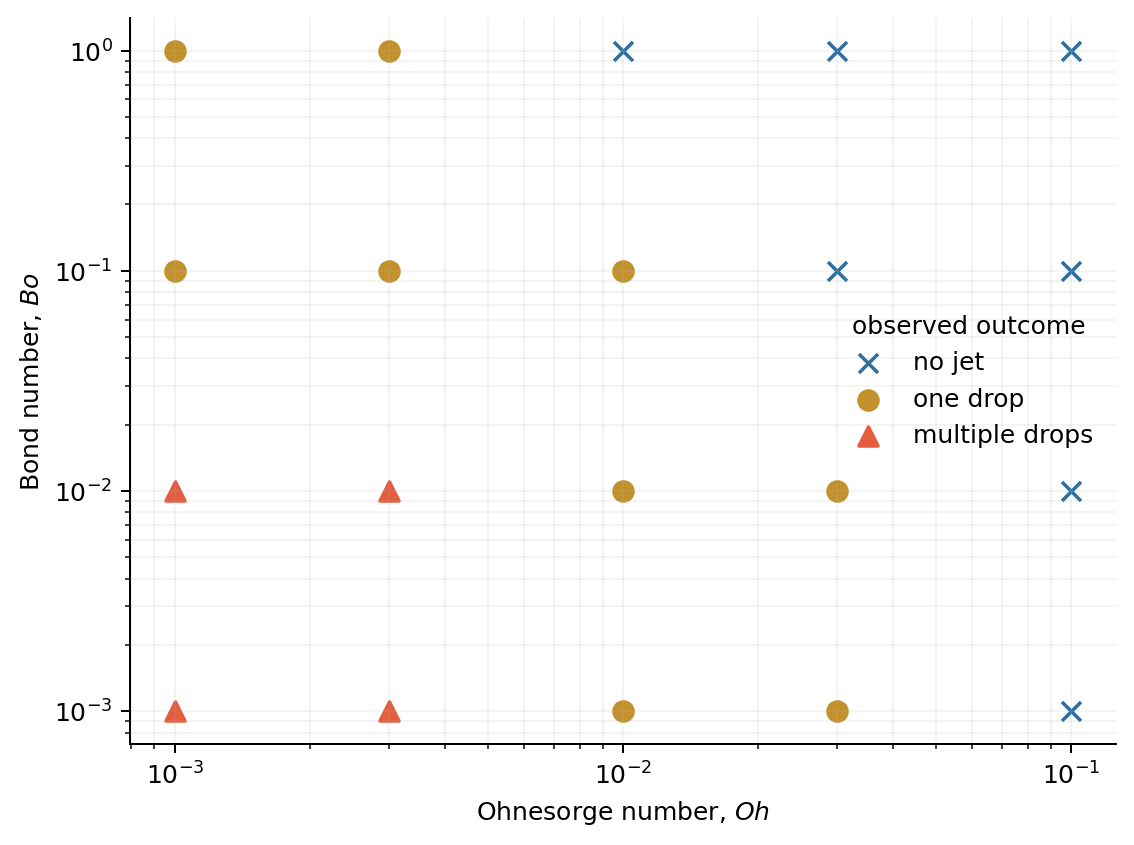
The reference figure uses:

• log \(Oh\) and \(Bo\) axes;
• both marker shape and colour;
• categorical points without connecting lines;
• a legend whose order is deliberate.

Check the source table when points overlap. A rendered figure is a projection, not the canonical case inventory.

The points preserve the supplied case classifications. Empty space is not silently converted into a smooth phase boundary.

Boundary temptation

It is easy to add:

contourf(interpolated_outcomes)

That would turn categories into an invented continuous scalar and allow the interpolator to choose a boundary. A boundary is warranted only when you state:

• the physical or statistical model;
• the encoding of categories;
• the interpolation or classifier;
• uncertainty;
• resolution and additional cases near the transition.

Until then, show the samples.

Verify

The reference checks cover:

1. duplicate case IDs;
2. an unknown category;
3. a zero \(Oh\);
4. all three categories appearing in the legend;
5. input row order not changing the plotted category counts.

For a research map, add a manifest:

Case	Parameters	Source path	Status	Classifier	Reviewer
c001	\(Oh=10^{-3}, Bo=10^{-3}\)	…	complete	multiple drops	…

Human classification is acceptable if the rule and review are explicit.

Extend

Choose one transition region and propose the next five cases. Do not fill a rectangular grid automatically. Select cases that discriminate between plausible boundaries or reveal hysteresis and resolution dependence.

Then write a function that outputs the proposed parameter table without submitting anything.

Reflect

A good regime map is not the prettiest interpolation. It is the smallest visual summary that preserves the evidence needed to challenge every category and boundary.