08 · Numerical results require verification

A solver can converge to the wrong equation. A time step can be stable but inaccurate. A smooth figure can preserve a systematic error perfectly.

Decision: what independent evidence makes the numerical result credible?

Output: an analytic, conservation, convergence, or cross-code check.

Frame

For a numerical derivative, three questions are different:

1. Did the program run?
2. Did the discrete algorithm converge?
3. Did we discretise the intended mathematical quantity?

Passing question one says almost nothing about two and three.

Predict an error law

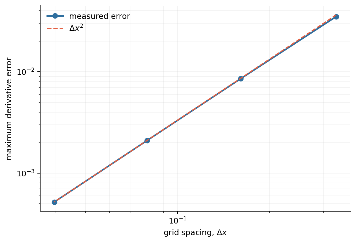
For a second-order centred difference, the error should scale as

\[ E(\Delta x) \propto \Delta x^2 \]

while the solution is smooth and roundoff has not taken over.

Run several grid spacings, calculate an error norm against an analytic derivative, and inspect:

observed_order = np.log(error_coarse / error_fine) / np.log(2)

An observed order near two is evidence about the implementation. It is not a proof that the model is physically appropriate.

The independent analytic derivative of \(\sin x\) exposes the expected second-order error law before roundoff dominates.

Use independent checks

Analytic solution or limit

Choose a case with a known result: a polynomial derivative, exponential decay, or low-parameter asymptote.

Conservation

Track mass, momentum, or energy budgets with the correct sources and fluxes. Plot the residual, not only the main observable.

Resolution study

Change grid spacing, time step, solver tolerance, or domain size. The quantity of interest should settle within an accuracy relevant to the claim.

Cross-implementation comparison

Compare Python with a C or Basilisk implementation on the same inputs and a common grid. Agreement is useful only if the implementations are sufficiently independent.

Regression

Freeze a trusted reduced result and fail CI if it changes unexpectedly. Regression detects change; the earlier checks establish trust.

Residual is not error

A small nonlinear-solver residual means the discrete equations have been solved to tolerance. It does not measure:

• discretisation error;
• modelling error;
• incorrect boundary conditions;
• wrong nondimensionalisation;
• an error shared by residual and solution.

Use precise language: “the residual fell below \(10^{-8}\)” is different from “the solution is accurate to \(10^{-8}\)”.

Compare like with like

Before comparing two codes:

• align units and nondimensional variables;
• match geometry and boundary conditions;
• interpolate onto a declared common coordinate if necessary;
• compare the same observable;
• separate interpolation error from solver error.

The public Contact-line-subgrid-modeling project contains the right advanced idea: solve the same GLE in Python and C, align the grids, and compare errors. Its legacy globals and hard-coded paths are also useful reminders that a sound verification idea still needs maintainable implementation.

Fit windows are part of the result

A power-law exponent depends on:

• the chosen window;
• resolution and noise;
• whether the asymptotic regime has begun;
• whether another regime contaminates the data.

Record fit-window metadata beside the reduced result. Do not tune a window until the desired exponent appears and then omit the tuning history.

The public SingularJets2026 capsule shows the mature pattern: exact regression tests, metadata-backed windows, checksums, a locked Python environment, and an offline rebuild.

Verify

Complete Exercise 08:

1. differentiate \(\sin x\) on 20, 40, 80, and 160 points;
2. compute the maximum error;
3. estimate the observed order;
4. plot error against spacing on log–log axes;
5. explain where boundary and roundoff errors enter.

Then compare it with Exercise 03 and deliberately use a first-order one-sided rule at both boundaries. Which error norm reveals the boundary damage most clearly?

Reflect

For a result you currently trust, name the strongest independent check. “It looks right” and “another student got something similar” are starting points, not verification.